Flux-based hierarchical organization of Escherichia coli's metabolic network
Semidán Robaina-Estévez* and Zoran Nikoloski
Systems Biology and Mathematical Modeling Group. Max Planck Institute of Molecular Plant Physiology. Bioinformatics Group, University of Potsdam, Potsdam, Germany
This notebook contains the workflow used to generate the results presented in the accompanying paper: Robaina-Estévez and Nikoloski (2019). Specifically, we find and analyze the flux-ordered reaction pairs in E. coli's genome-scale metabolic model iJO1366 under growth in three carbon sources: glucose, glycerate and acetate. Further, we reconstruct the directed acyclic graph (DAG) which represents the flux-order relation and analyze which metabolic subsystems are predominant in each graph level. Finally, we evaluate whether diverse experimental measurements—such as ${}^{13}\mathrm{C}$-estimated fluxes, protein and transcript levels—reflect the predicted flux-order relation. For more detailed information about the results and the methods employed we refer the reader to the accompanying paper. Let's get started!
General notes:: First, there are several interactive figures in the notebook. These figures require the notebook to be trusted to work — unless you are seeing this notebook as a web page, in this case ignore this message. All interactive figures have been generated using modified code from Jupyter's ipywidgets, see repository. Second, some of the computations in this notebook can take time, however, it is not necessary to run the notebook to see the interactive figures, since they work even without a kernel. The notebook requires the python libraries found in requirements.txt in order to be run.
*corresponding author: hello@semidanrobaina.com
# Import required libraries
import pandas as pd
import numpy as np
import copy
import networkx as nx
from scipy import cluster, spatial
from matplotlib import pyplot as plt
from cobra.flux_analysis.variability import find_essential_reactions
from matplotlib_venn import venn3_unweighted
from IPython.display import display, Markdown, HTML
plt.style.use('seaborn')

# Import own modules
from Data_module import DataParser
from Model_module import Model
from Order_module import FluxOrder, DataOrderEvaluator, getFluxOrderDataFrame
import Helper_methods as hm
import Plot_methods as pm

carbonSources = ['glucose', 'glycerate', 'acetate']
n_sources = len(carbonSources)
workDir = '/Documents/Projects/Ordering_of_Fluxes'
%matplotlib inline
1. The flux order relation in Escherichia coli
In this first section, we begin by importing the iJO1366 model and setting the correct environmental conditons for the three carbon sources evaluated: glucose, glycerate and acetate. We then continue finding the flux-ordered reaction pairs of iJO1366 in the three carbon sources. Next, we compare the sets of flux-ordered reactions among carbon sources, to evaluate to which extent the flux order relation depends on environmental conditions. Finally, we will analyze the overlap between the sets of flux-ordered reaction pairs and flux-coupled reaction pairs since they do share some properties.
1.1. Creating model instancies for the three carbon sources
We begin by importing the iJO1366 model into the cobrapy toolbox, we will process the model to remove blocked reactions—i.e., reactions that cannot carry flux in any steady state—and to split reversible reactions into the two possible directions: forward and backward (here tagged as reverse). The class Model found in Model_module of this study provides all the required methods. In all three cases, we simulate the growth of E. coli in a minimal medium with a single carbon source, to this end, we neglect the import of any organic compound besides the carbon source and cobalamine (vitamin B12), since E. coli cannot synthetize it. We set the maximum carbon source uptake flux to be 20 $\mathrm{mmol.L}^{-1}.\mathrm{min}^{-1}$, and constraint the flux through the biomass reaction to be at least 95% of the maximum flux possible under the given constraints. Note that we include an additional environmental condition, all, in which the model is allowed to take any of the three carbon sources here evaluated, we will use this additional setting later on.
# Prepare Models for the three carbon sources
iJO1366 = {}
temp = Model(fileName='iJO1366.json', workDir=workDir + '/Models/iJO1366')
for carbonSource in carbonSources + ['all']:
    print(' ')
    print('Preparing model for carbon source: {}'.format(carbonSource))
    temp.setCarbonSource(carbonSource, uptakeRate=20, fractionOfBiomassOptimum=0.95)
    iJO1366[carbonSource] = copy.deepcopy(temp)
1.2. Finding flux-ordered reaction pairs
Now that we have prepared the iJO1366 model, we proceed to find all flux-ordered reaction pairs for the three carbon sources. That is, for each reaction pair $r_i,r_j$ in the model we want to test whether their fluxes satisfy $v_i \geq v_j, \forall v \in C = \{v:Sv=0,v_{min} \leq v \leq v_{max}\}$ (see accompanying paper for details). To this end, we employ a simple linear program which maximizes the flux ratio of a pair of reactions. Specifically, we start with the linear-fractional program
\begin{align} \begin{aligned} &z_{max} = \max_v \; \frac{v_j}{v_i} \\ &\mathrm{s.t.} \\ &Sv=0 \\ &v_{min} \leq v \leq v_{max} \end{aligned} \label{eq:1} \end{align}and apply the Charnes-Cooper transformation to obtain the linear program
\begin{align} \begin{aligned} &z_{max} = \max_{w,t} \; w_j \\ &\mathrm{s.t.} \\ &Sw = 0 \\ &w_i = 1 \\ &tv_{min} \leq w \leq tv_{max} \\ &t \geq 0 \end{aligned} \label{eq:2} \end{align}in which $w_j = \frac{v_j}{v_i}$. A reaction pair is then flux-ordered if $z_{max} \leq 1$. However, repeating this process for all possible reaction pairs in the model is computationally intensive, since the number of pairs grows as $\frac{1}{2} n(n-1)$ where $n$ is the number of reactions in the model. To speed up the computation time, we first apply a less computationally expensive process in which we discard reaction pairs that cannot be flux-ordered. Specifically, we draw a number of random flux samples for all reactions in the model, then we discard reaction pairs for which in at least one of the samples the flux order relation is not satisfied. Additionally, we can further narrow down the set of candidate pairs through flux variability analysis (FVA) as follows . First, we compute the flux distributions which maximize each reaction flux in the model. Let $w$ be the flux distribution that maximizes the flux through $r_j$, i.e. $w_j = v_{max(j)}$. If $v_i \geq v_j$ truly holds, then $w_j \leq w_i$, i.e., even at the flux distribution that maximizes $v_j$, reaction $r_i$ carries a larger or equal flux $w_i$. We call the remaining reaction pairs candidate flux-ordered, which we further test with the previous linear program to assess whether or not they really are flux-ordered.
As an example, let's find the candidate flux-ordered pairs for the case of growth in minimal medium with glucose as the sole carbon source. We will omit the FVA filter since it requires a working installation of R as well as of the rpy2 python library and the Gurobi solver, which are not required to reproduce the rest of the results in this notebook. However, we did employ the FVA filter when computing the supplied flux order adjacency matrices which will be uploaded later on.
# Find candidate flux-ordered reaction pairs
iJO1366['glucose'].findCandidatePairs(nsamples=5000, fva_filter=True)
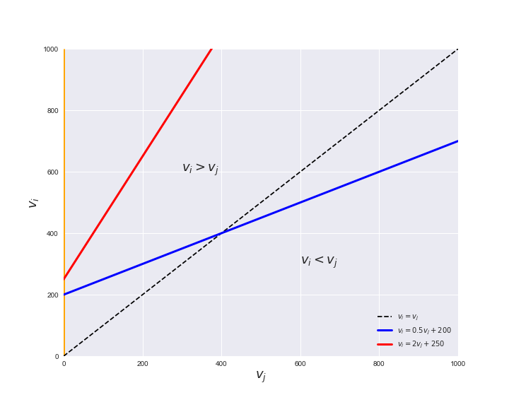
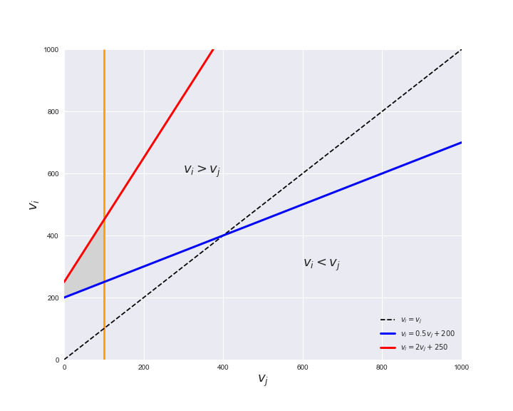
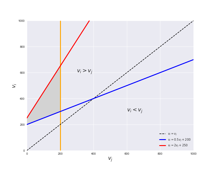
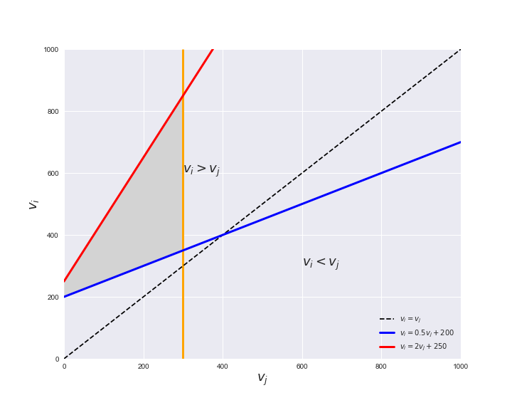
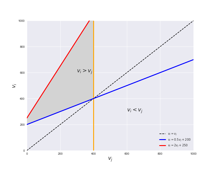
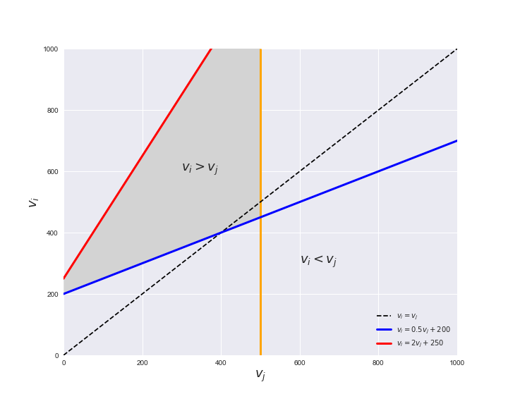
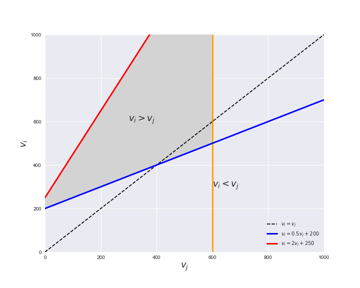
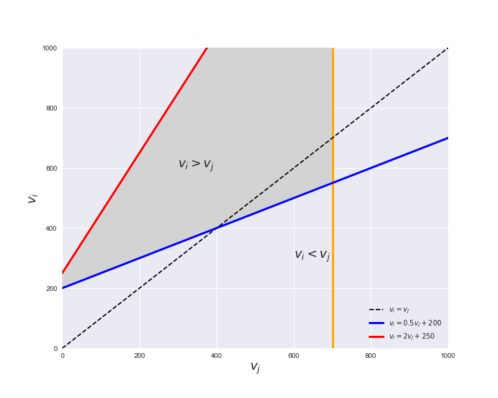
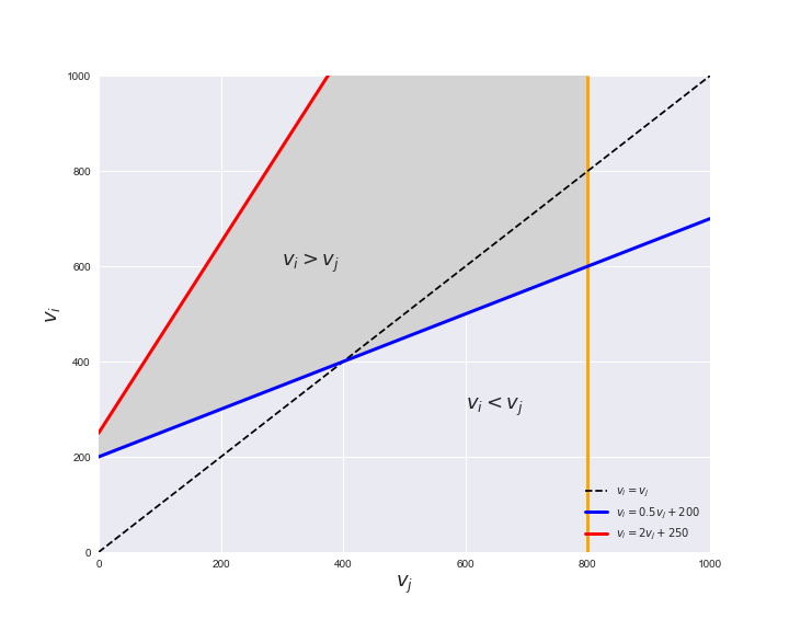
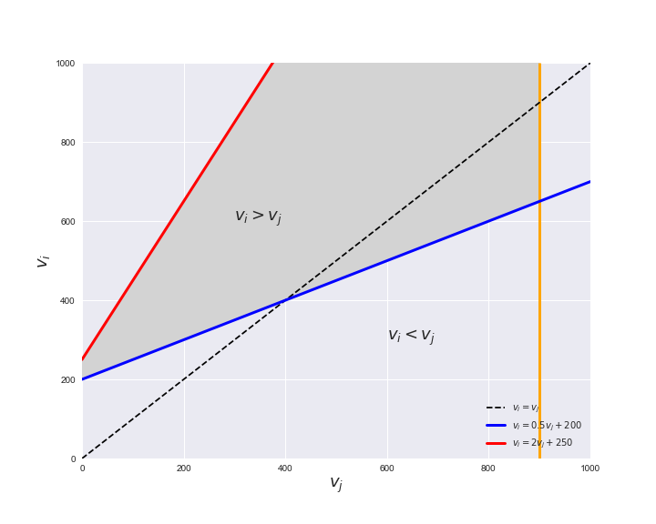
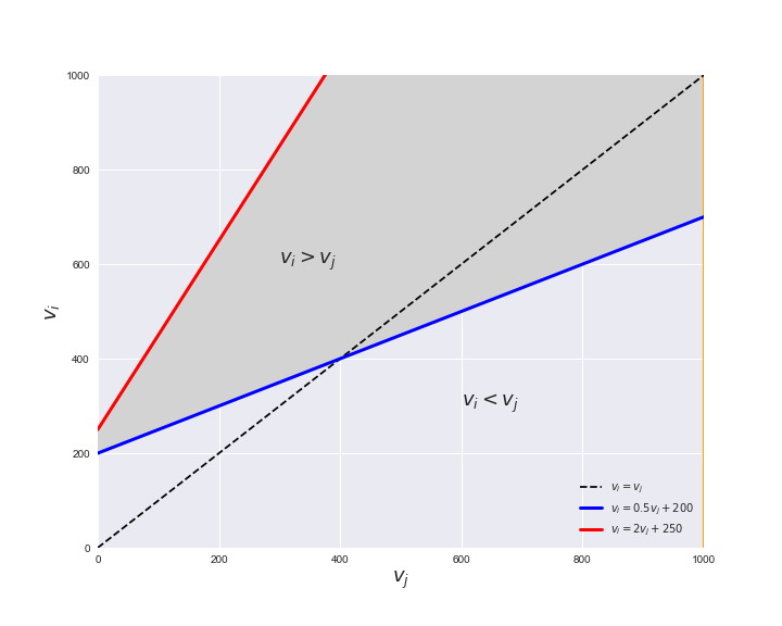
Unlike flux coupling relations, the flux order relation depends on the flux bounds of each reactions. For instance, in the following interactive figure, we depict the steady-state flux space for two reactions $r_i, r_j$, which is delimited by the two constraints drawn in red and blue. Every flux pair above the dashed line representing $v_i = v_j$ satisfies $v_i > v_j$. Now, the adjustable golden line depicts the flux upper bound of reaction $v_j$. We see that only when the upper bound reaches a value of 400 the reaction pair becomes flux-ordered, since the feasible region, shaded in grey, lays entirely above the dashed line. This dependency of the flux-order relation of the flux bounds is also the reason why different sets of flux-ordered pairs may be found under different simulated conditions, such as the three carbon sources evaluated here.
# Plot example
pm.plotOrderExample(min_flux=0, max_flux=1000, range_step=100,
                    default_value=600, description='$v_j^{ub}$')
Now that we have found the candidate flux-ordered pairs, we are ready to evaluate which of the candidates are truly ordered. Solving the previously presented linear program for each of the candidate pairs is an embarrassingly parallel task, hence, we employ the Gurobi in a parallel setting using the R programming language. To this end, we can call the supplied R function get_flux_orders, found in Rfunctions.R, through python using the rpy2 module
fluxOrders_A = get_flux_orders(S, lb, ub, candidatePairs)
which returns the adjacency matrix of the directed acyclic graph representing the flux order relation, that is, the entry $a_{ij} = 1$ if $v_i \geq v_j$ and $a_{ij} = 0$ otherwise. Alternatively, we directly call the function within R. To this end, we need to export the stoichiometric matrix $S$, flux bounds $lb, ub$ and the array containing the candidate pairs to csv using the exportToCSV method of the Model class, that is, we would call
model_attributes = ['S', 'lb', 'ub', 'candidatePairs']
for carbonSource in carbonSources:
    iJO1366[carbonSource].exportToCSV(attributes=model_attributes, directory=path_to_directory)
which would create the files: 'S_carbonSource.csv', 'ub_carbonSource.csv', 'lb_carbonSource' and 'candidatePairs_carbonSource.csv'. We would proceed to import the csv files in R and call the function (see the documentation within 'Rfunctions.R' for an example). While this procedure is a bit more cumbersome, calling get_flux_orderes directly within R increases performance. Finding all flux-ordered pairs (directly within R) took around 5 hours using a laptop with 4 cores (8 threads) for each carboun source. To accelerate this process, we will employ the already computed adjacency matrices for each of the three carbon sources.
# Upload adjacency matrices for each carbon source
iJO1366_A = {}
for carbonSource in carbonSources:
    iJO1366_A[carbonSource] = np.genfromtxt(workDir + '/Data/Models/iJO1366/iJO1366_AdjMat_'
                                            + carbonSource + '.csv', delimiter=',')
1.3. Comparing the flux-ordered pairs among the three carbon sources
Here, we analyze the similarities and differencies among the sets of flux-ordered reaction pairs corresponding to the three carbon sources. First of all, we will compare the total number of flux-ordered pairs, then, generate a Venn diagram to show the extent to which flux-ordered reaction pairs are shared among carbon sources. We will also compute the Jaccard distance between each set of flux-ordered pairs and plot a dendrogram to further visualize the differences. Let's plot the total number of flux-ordered pairs, then.
# Count number of ordered pairs per carbon source
number_pairs, ordered_pairs = {}, {}
for carbonSource in carbonSources:
    ordered_pairs[carbonSource] = set(np.where(iJO1366_A[carbonSource].flatten() == 1)[0])
    number_pairs[carbonSource] = len(ordered_pairs[carbonSource])
number_pairs['average'] = np.mean([number_pairs[source] for source in carbonSources])


# Plot bar plot with total counts
n_rxns = iJO1366['all'].numberOfReactions

number_total_pairs = 0.5 * n_rxns * (n_rxns - 1)
plt.figure(figsize=(10, 6))
bars = plt.bar(range(n_sources + 1), number_pairs.values(),
               width=0.5, tick_label=list(number_pairs.keys()))
plt.xticks(fontsize=18)
plt.ylabel('counts', fontsize=18)
plt.title('Number of flux-ordered pairs', fontsize=18, pad=20)

# Add counts above the bars
for bar in bars:
    height = bar.get_height()
    bar_text = '%.1f' % height + ' (' + '%.2f' % (100 * height / number_total_pairs) + r'%)'
    plt.text(bar.get_x() + bar.get_width()/2.0,
             height, bar_text, ha='center', va='bottom', fontsize=14)


plt.show()

We see that glucose is the carbon source that produces the least number of flux-ordered reaction pairs, while acetate the largest number. While the number of flux-ordered pairs is quite large on average, it only supposes a 5.4% of the total number of reaction pairs in the iJO1366 model. Let's now delve into the differences and similarities among the carbon sources. We begin by constructing a Venn diagram to visualize the intersection structure among the three sets.
# Plot Venn diagram depicting sets of flux-ordered pairs
plt.figure(figsize=(8, 8))
plt.title('Intersections of ordered pairs among carbon sources', fontsize=18)
venn3_unweighted(ordered_pairs.values(), ordered_pairs.keys())
plt.show()

# Fraction of shared ordered pairs per carbon source
number_shared_pairs = 94071
print('Fraction of shared ordered pairs per carbon source:')
for carbonSource in carbonSources:
    print('{}: {:.2f}%'.format(carbonSource, 100 * (number_shared_pairs / number_pairs[carbonSource])))
We can see in the Venn diagram that a large number of flux-ordered reaction pairs are shared among the three carbon sources. However, with respect to the total number of pairs of each carbon source, we see that, in the case of glucose, the set of shared pairs supposes as much as 91.86% of the total pairs, while this figure is lower for acetate and glycerate, 72.49% and 75.33%, respectively. That is, the majority of the flux-ordered pairs in the glucose escenario are contained in the other two carbon sources. Additionally, acetate and glycerate do share a marked number of flux-ordered pairs, altough acetate is the carbon source with the largest number of exclusice flux-ordered pairs.
Altogether, the previous results indicate that the sets of flux-ordered pairs generated under acetate and glycerate seem to be more similar to one another than to the ones generated under glucose, in fact almost a superset of the latter. We can further visualize the similarities between carbon sources through a dendrogram. We will use the Jaccard index as a distance between the sets of flux-ordered pairs among carbon sources.
# Reconstruct the Jaccard distance matrix
iJO1366_D = pd.DataFrame(np.zeros((n_sources, n_sources)),
                         index=carbonSources, columns=carbonSources)
for carbonSource1 in carbonSources:
    for carbonSource2 in carbonSources:
        dist = spatial.distance.jaccard(
            iJO1366_A[carbonSource1].flatten(), iJO1366_A[carbonSource2].flatten())
        iJO1366_D[carbonSource1][carbonSource2] = dist

# Plot dendrogram of Jaccard distance
Z = cluster.hierarchy.linkage(1 - iJO1366_D.values, 'single')
plt.figure(figsize=(10, 6))
plt.title('Jaccard distance among flux-ordered sets', fontsize=18, pad=20)
plt.ylabel('distance', fontsize=18)
cluster.hierarchy.dendrogram(Z, labels=iJO1366_D.columns)
plt.show()

1.4. Analyzing the overlap with flux coupling relations
Flux coupling relations establish constraints between the activity patterns, i.e., whether or not they carry non-zero flux, of reaction pairs in a genome-scale model. Specifically, two reactions, $r_i, r_j$ are fully or partially coupled if the two reactions are always active or always inactive in any steady state. With the difference that fully coupled reactions also have a fixed flux ratio when active, i.e., $\frac{v_i}{v_j} = \alpha$ for a fixed $\alpha$. Both, the fully coupled relation, represented as $r_i \Leftrightarrow r_j$, and the partially coupled relation, represeted as $r_i \leftrightarrow r_j$ are symmetric. Contrary, in the directional coupling relation, one (leading) reaction controls the activation state of another reaction, thus this relation is asymmetric, i.e., $r_i \rightarrow r_j$.
Flux coupling relations share some similarities with the flux order relation. To start with, they are both a consequence of network topology and the steady-state constraint. Further, the directional coupling relation is also asymmetric and hence also induces a partially ordered set (i.e., a hierarchy) which can be represeted by a DAG. (The other two coupling relations: full and partial, are symmetric and thus cannot form a DAG.) However, contrary to the flux-order relation, flux-coupling relations are not affected by the particular flux bounds impose on the reactions, that is, as long as reactions are not rendered inactive by the flux bounds. Because of this, we only generate one set of flux-coupled reaction pairs which is the same for the three carbon sources.
Here, we will study to which extend flux coupled reaction pairs overlap with the identified flux-ordered pairs. First, we need to find the flux couple relations in our model, iJO1366. F2C2 is an efficient tool for this task. Unfortunately, it's been only implemented in MATLAB. For this reason, we need to upload here a pre-computed matrix (obtained through F2C2 in MATLAB) which identifies the flux coupled pairs among all reaction pairs in iJ1366. The entry code is the following, for each reaction pair $r_i, r_j$, we have
- $a_{i,j} = 0$ -> uncoupled
- $a_{i,j} = 1$ -> fully coupled
- $a_{i,j} = 2$ -> partially coupled
- $a_{i,j} = 3$ -> directionarlly coupled
After obtaining the sets of flux coupled reaction pairs, we will compute the fraction of flux-ordered pairs that are also fully, partially and directionally coupled. Similarly, we will compute the fraction of partially and directionally coupled pairs that are also flux-ordered. Note that all fully coupled pairs are flux-ordered because their ratio is fixed. First, let's compare the sizes of the sets of flux-ordered and flux-coupled reactions.
# Upload flux coupling relations matrix
iJO1366_fctable = np.genfromtxt(
   workDir + '/Data/Models/iJO1366/fc' + 'iJO1366' + '.csv', delimiter=',')

# Compute fraction of coupled pairs (all three types)
nrxns = np.size(iJO1366_fctable, 0)
number_reaction_pairs = 0.5 * nrxns * (nrxns - 1)
number_coupled_pairs = (len(np.where(iJO1366_fctable > 0)[0]) - nrxns) / 2
coupled_fraction = 100 * (number_coupled_pairs / number_reaction_pairs)

print('There are {coupled} coupled pairs out of a total of {total}. That is a fraction of {fraction:.2f}%'.format(
    coupled=int(number_coupled_pairs), total=int(number_reaction_pairs), fraction=coupled_fraction))
To begin with our comparison, we see that there are more flux-ordered reaction pairs than flux-coupled reaction pairs. Remember, that we saw before that, on average, the fraction of flux-ordered pairs across carbon sources was 5.40%, while the fraction of all types of flux-coupled pairs (for the three carbon sources) is 1.91%. Let's now look at the overlap between the sets of flux-ordered and flux-coupled reactions. We will plot pie charts for each carbon source depicting the fraction of flux-ordered reactions that are also fully, partially and directionally coupled.
# Find fractions and plot pie charts
fig, axs = plt.subplots(nrows=1, ncols=3, sharex=False, sharey=False, figsize=(16, 6))
plt.suptitle('Flux couplings in ordered pairs', fontsize=18)
colors = [ ['#cbcbcb', '#005b88', '#0572a8', '#0d94d7'],
          ['#cbcbcb', '#237506', '#299404', '#35ba07'],
          ['#cbcbcb', '#cf7e04', '#e88f09', '#ff9900'] ]

coupled_ordered, iJO1366_Orders = {}, {}
for i, carbonSource in enumerate(carbonSources):
    iJO1366_Orders[carbonSource] = FluxOrder(iJO1366[carbonSource],
        iJO1366_A[carbonSource], iJO1366_fctable)

    # Get fraction of coupled pairs that are also ordered
    coupled_ordered[carbonSource] = iJO1366_Orders[carbonSource].evaluateFluxCouplingRelations(
        axs[i], colors[i])['fraction ordered coupled']

plt.subplots_adjust(hspace=0)
plt.show()

We see in the pie charts that the majority of flux-ordered pairs are not flux-coupled in all three carbon sources, with acetate being the carbon source in which less ordered pairs are also coupled. Therefore, the flux order relation is not contained in the flux coupling relations. Further, almost all flux-ordered and flux-coupled pairs are directionally coupled in all three cases. Let's see next what fraction of partially and directionally coupled pairs are also flux-ordered.
# Get fraction of coupled pairs that are also ordered
df = pd.DataFrame.from_dict(coupled_ordered)
display(HTML(df.to_html()))
print('Mean proportion of coupled pairs that are ordered across carbon sources:')
for coupling_type in ['partial', 'directional']:
    print('{} and ordered: {:.2f}%'.format(coupling_type, np.mean(
        [coupled_ordered[source][coupling_type] for source in carbonSources])))
In fact, the majority of both directionally and partially coupled pairs are also flux-ordered (and all fully flux-coupled pairs by definition). Specifically, on average across carbon sources, 92.7% of partially coupled and 81.7% of directionally coupled pairs are also flux-ordered. Thus the set of flux-order reactions contains the majority of flux-coupled reactions.
2. Analyzing the flux order DAG.
In this section, we reconstruct the flux order directed acyclic DAGs for the three carbon sources from the adjacency matrices obtained before. We first analyze some basic features of the DAGs such as the number of levels in the hierarchy and the distribution of reactions per graph level. We include an example of a flux-ordered reaction chain obtain from one of the DAGs. We then proceed to display the distribution of reaction metabolic subsystems and macrosystems per graph level.
2.1. Reconstructing the flux order DAG
Let's start by extracting all the reactions in each of the levels of the flux order graph and per each carbon source. We will then plot a histogram depicting the number of reactions per level and carbon source
# Generate the graph of the Hasse diagram through networkx
Graph_Levels, iJO1366_Orders_DAG = {}, {}
for carbonSource in carbonSources:
    iJO1366_Orders_DAG[carbonSource] = iJO1366_Orders[carbonSource].getGraph()
    Graph_Levels[carbonSource] = iJO1366_Orders_DAG[carbonSource].getGraphLevels()
rxn_distribution = pm.plotNumberOfReactionsPerGraphLevel(Graph_Levels)

We can see that the first levels, i.e. those in which reactions tend to impose an upper flux bound to the larger number of reactions, accumulate the majority of reactions involved in a flux order relation. Additionally, we observe no large differences among carbon sources. Acetate produces a graph with an additional level. Let's now plot a stacked bar plot depicting the representation of each metabolic macrosystem in the entire set of ordered reaction pairs for each carbon source.
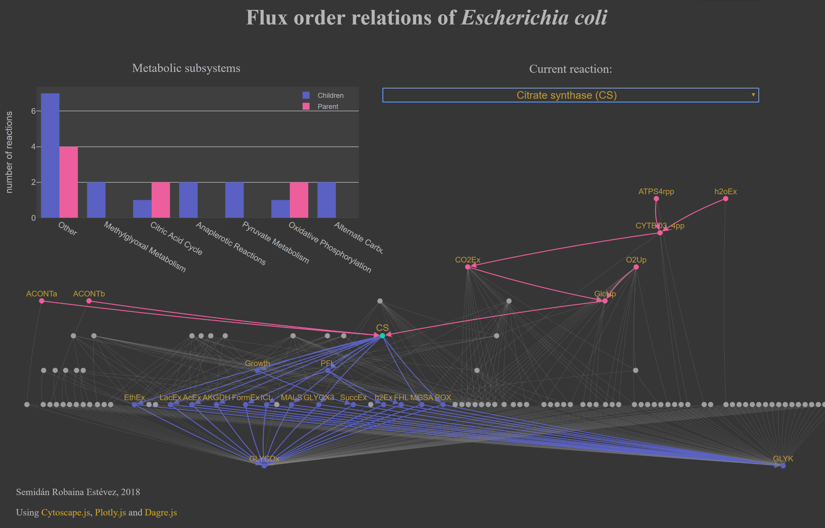
2.2. An interactive flux order DAG of E. coli's core network
The flux order DAG obtained using the complete metabolic network in iJO1366 is too large to be visualized in any meaningful way. To help with this issue, we prepared a a flux order DAG of a smaller metabolic network, EColiCore2 which contains the core part, i.e., the central carbon metabolism, of the iJO1366 model. Additionally, EColiCore2 maintains the same solution space at steady state (hence, same flux ordered reaction pairs) as iJO1366. For an interactive app of the flux order DAG of E. coli's core metabolic network under growth on glucose click on the following image:
2.3. An illustration of a flux-ordered chain
The flux-order relation is transitive, that is, for any two reaction pairs $r_i, r_j$ and $r_j, r_k$ with $i \neq j \neq k$, $v_i \geq v_j, v_j \geq v_k \implies v_i \geq v_k$. Hence, the transitivity of the flux order relation implies the formation of flux-ordered chains of reactions, in which the first reaction always has a flux value which is greater of equal than those downstream. Let's illustrate this property with the following example. We will extract a flux-ordered chain composed of 5 reactions from the flux orders DAG computed for the scenario with glucose as carbon source.
# Extract random ordered chain
example_source = 'acetate'
source_rxn_id = 'AKGDH'
chain_length = 5
orderedChain = iJO1366_Orders_DAG[example_source].getOrderedReactionChain(
    source=source_rxn_id, size=chain_length)

# Print reaction chain
rxn_names = str()
sample_chain_list = []
for multiple_rxn_ids in orderedChain:
    rxn_ids = multiple_rxn_ids.split(r'||')
    random_idx =  np.random.randint(len(rxn_ids))
    sample_chain_list.append(rxn_ids[random_idx])
    if len(rxn_ids) > 1:
        eq_rxn_names = '('
        for rxn_id in rxn_ids:
            eq_rxn_names += 'r_{' + rxn_id + '} = '
        eq_rxn_names = eq_rxn_names[:-3] + ')'
    else:
        eq_rxn_names = 'r_{' + rxn_ids[0] + '}'
    rxn_names += eq_rxn_names + r' \ge '

display(Markdown('__Ordered reaction chain__: <br>'+ '$' + rxn_names[:-4] + '$'))
We see that the root of this chain is reaction AKGDH (2-Oxogluterate dehydrogenase) while the sink, i.e., the last reaction in the chain, is reaction EAR121y (Enoyl-[acyl-carrier-protein] reductase). Hence, AKGDH must have the largest flux value and EAR121y the smallest of the chain in any steady state of the system. Note that some groups of reactions in the chain may carry equal fluxes (depicted within parentheses). These reactions are fully coupled among each other, with a couplig constant, i.e., a fixed flux ratio, of 1.
Let's now draw a random sample of flux distributions to certify that the flux levels of the reactions follow the flux-ordered chain structure presented above. To guarantee that the flux through the root reaction is non-zero in the same, we will constraint the lower flux bound of this reaction to a fraction of its theoretical maximum. We will then plot the sampled flux values for the reactions in the chain, to this end, we will pick one representative reaction from each group of fully coupled reactions
pm.plotFluxSampleOfOrderedChain(iJO1366[example_source], sample_chain_list)

We see that, as it must be, the sampled fluxes follow the order relation displayed in the flux-ordered reaction chain.
2.4. Representation of metabolic systems in the Hasse diagram
Until now, we have only cared about the similarities and differences in then numbers of flux-ordered reaction pairs as well as the sets themselves among carbon sources. Next, we will analyze which metabolic subsystems and macrosystems are represented in each level of the flux order DAG of each carbon source. While metabolic subsystems are those contained in the iJO1366 model, the macrosystems 8 broader metabolic categories which have been assigned to the subsystems of iJO1366 in this study (see Supplementary Table 1). We begin by computing the representation of the 8 macrosystems across graph levels for the three carbon sources. Specifically, we will look at the frequencies fo the macrosystems, i.e., the fraction of reactions in the DAG that have each macrosystem assigned, in the set of shared reactions among the three DAGs as well as the sets of exclusive reactions corresponding to each carbon source.
# Get sets of shared and exclusive reactions in the flux-order graph among carbon sources
shared_reactions, exclusive_reactions = hm.extractSharedAndExclusiveReactions(Graph_Levels)

# Get total reactions in the same structure as exclusive reactions
total_reactions = {}
max_number_of_levels = max([len(Graph_Levels[source]) for source in carbonSources])
for level in range(max_number_of_levels):
    total_reactions[level] = {}
    for carbonSource in carbonSources:
        try:
            reaction_list = Graph_Levels[carbonSource][level]
        except Exception:
            reaction_list = []

        total_reactions[level][carbonSource] = reaction_list

# Plot distribution of macrosystems
df = pm.plotTotalSystemsDistribution(iJO1366['all'], shared_reactions, exclusive_reactions, systemType='macrosystem')
display(HTML(df.to_html()))

Among the set of shared reactions, we see that Transport is by far the most frequent macrosystem, which is not surprising given that Transport is also the macrosystem with the largest number of reactions in the iJO1366 model. Transport is followed by Cell wall biosynthesis and Lipid metabolism. When we look at the sets of exclusive reactions for each carbon source, we already see differences in the representation of macrosystems. For instance, Transport is still the macrosystem with the largest number of exclusive reactions in the case of glucose and glycerate, but not in acetate. In the latter case, Lipid metabolism is the macrosystem with the largest number of reactions. Additionally, acetate is the only carbon source in which Cell wall biosynthesis is the second most common macrosystem in the set of exclusive reactions. Let's increase the resolution and plot the frequencies of macrosystems per graph level, i.e., the fraction of reactions in each level which have assigned the macrosystem, and carbon source next.
# Plot distribution of macrosystems and subsystems per graph level
interactive_fig = pm.plotLevelSubsystemsStatic(iJO1366['all'], total_reactions)
interactive_fig
graph level =
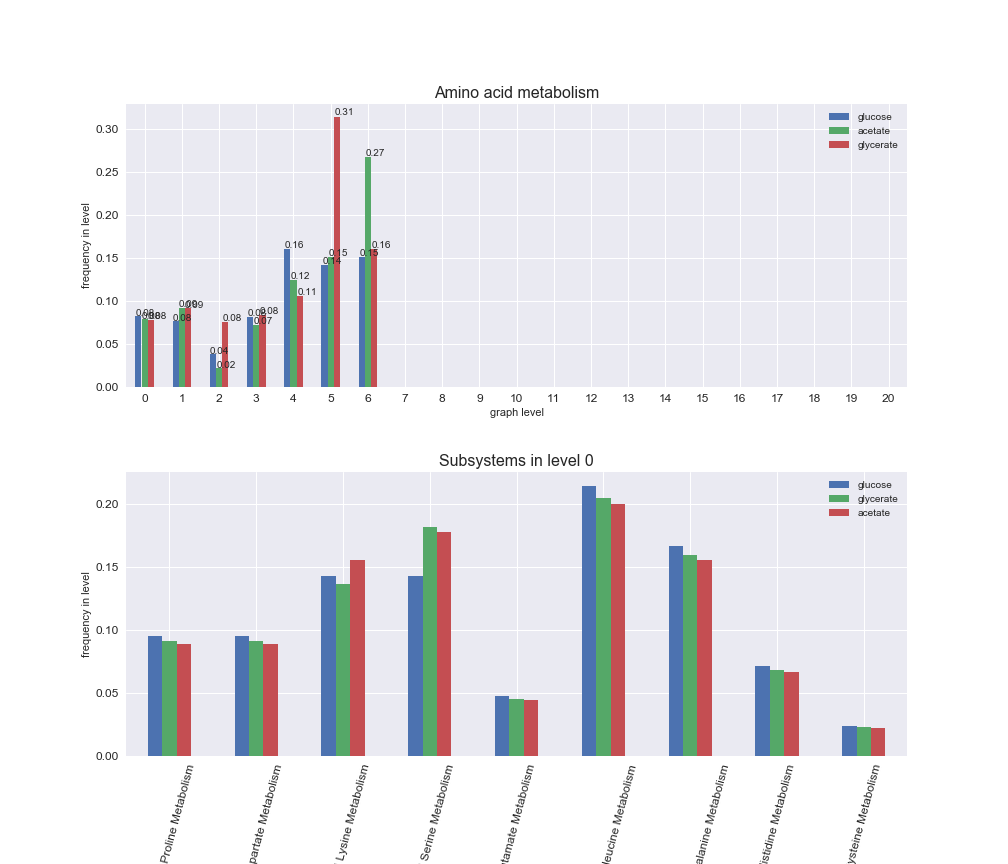

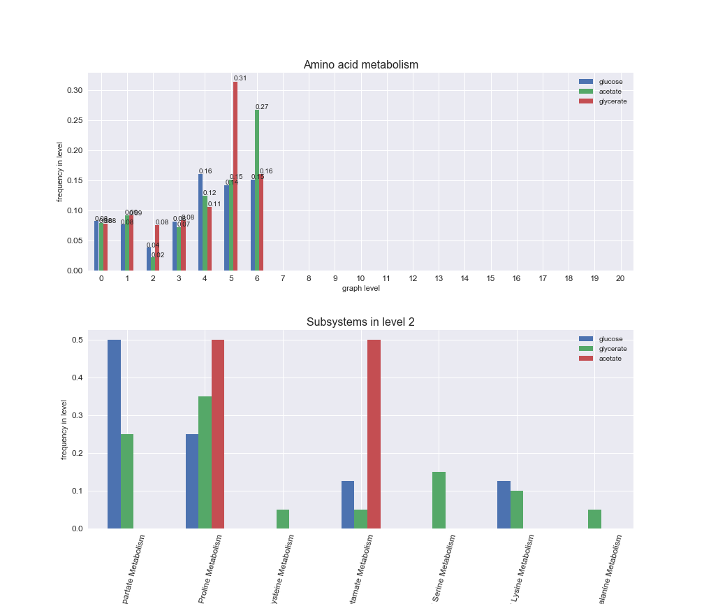
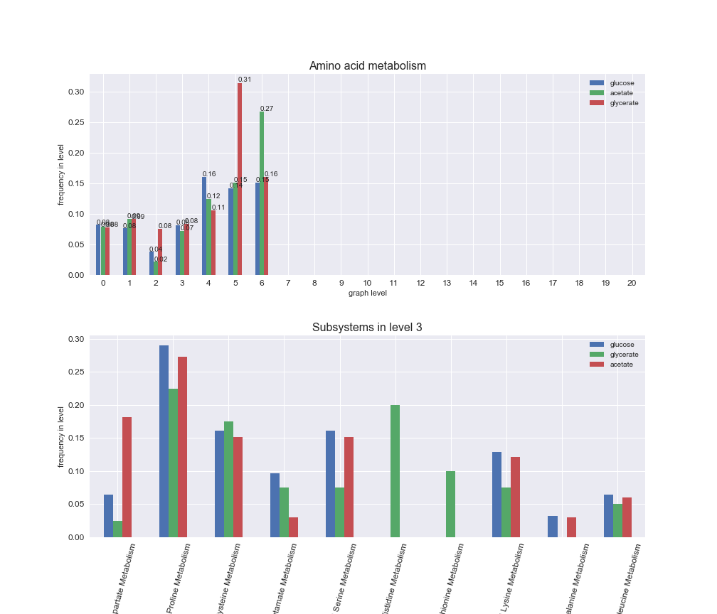
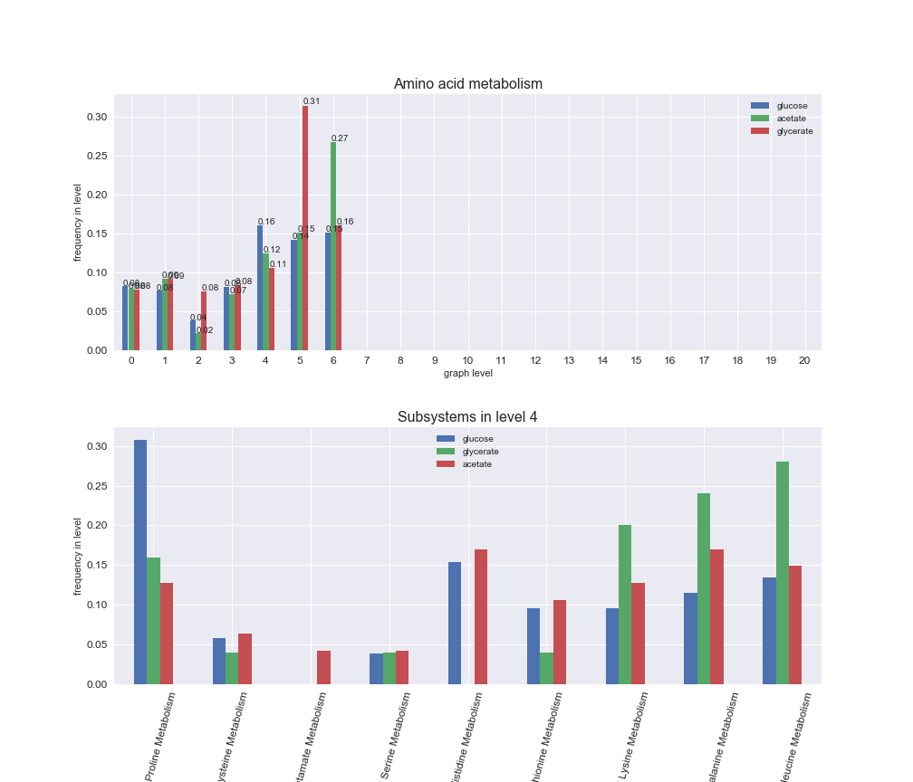
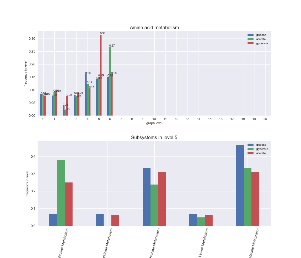
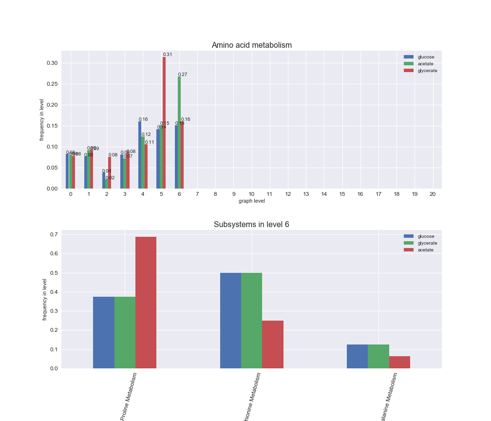


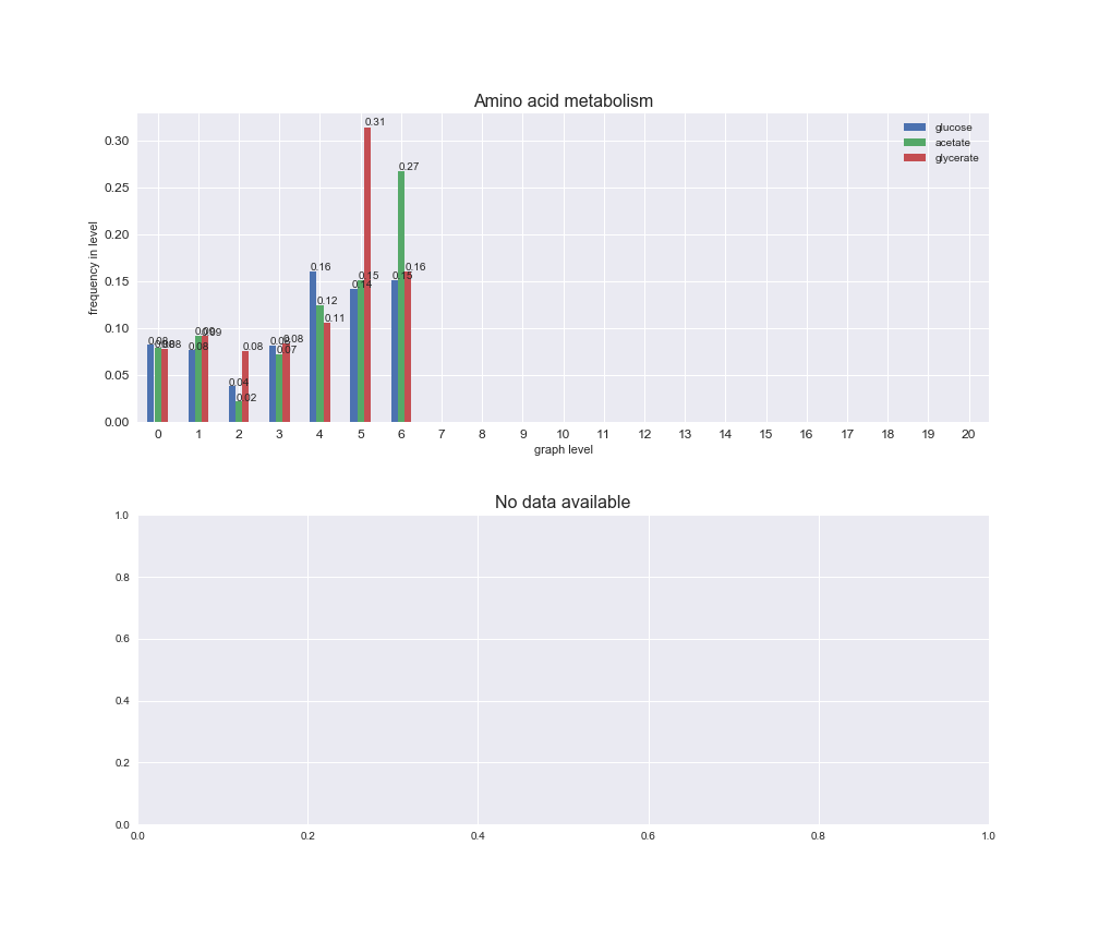


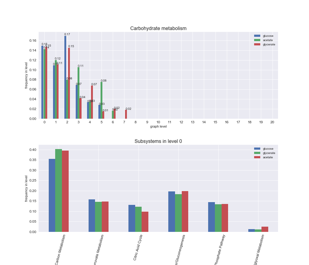
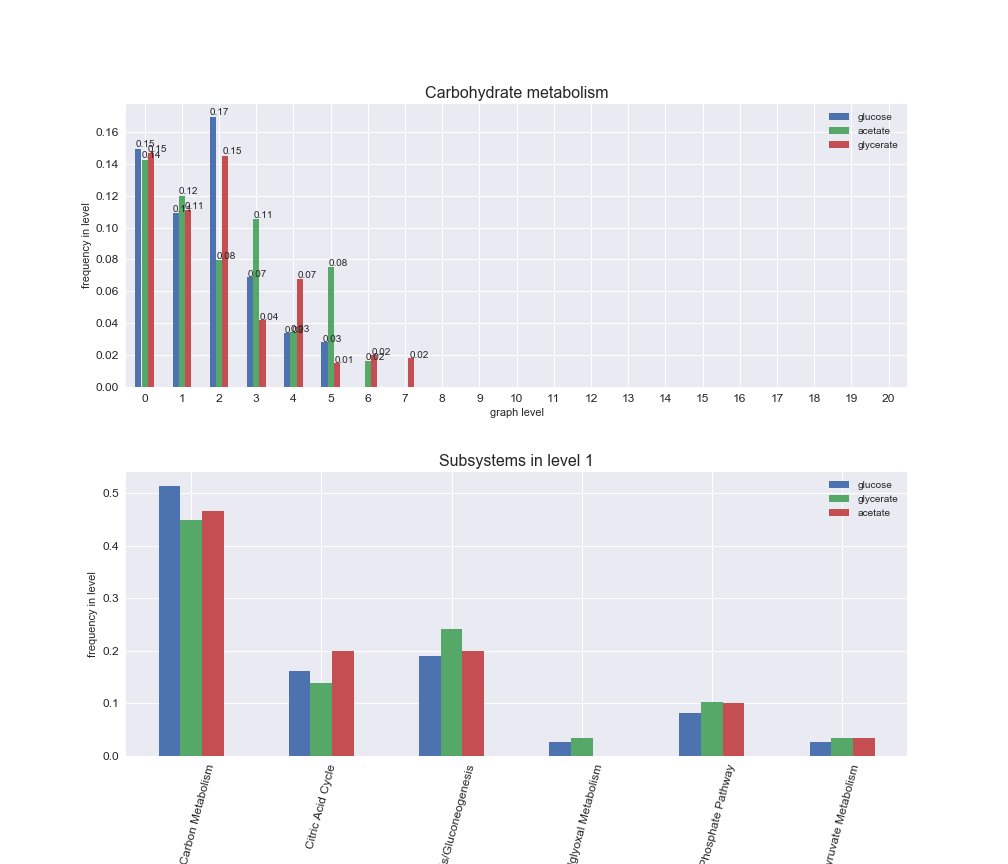
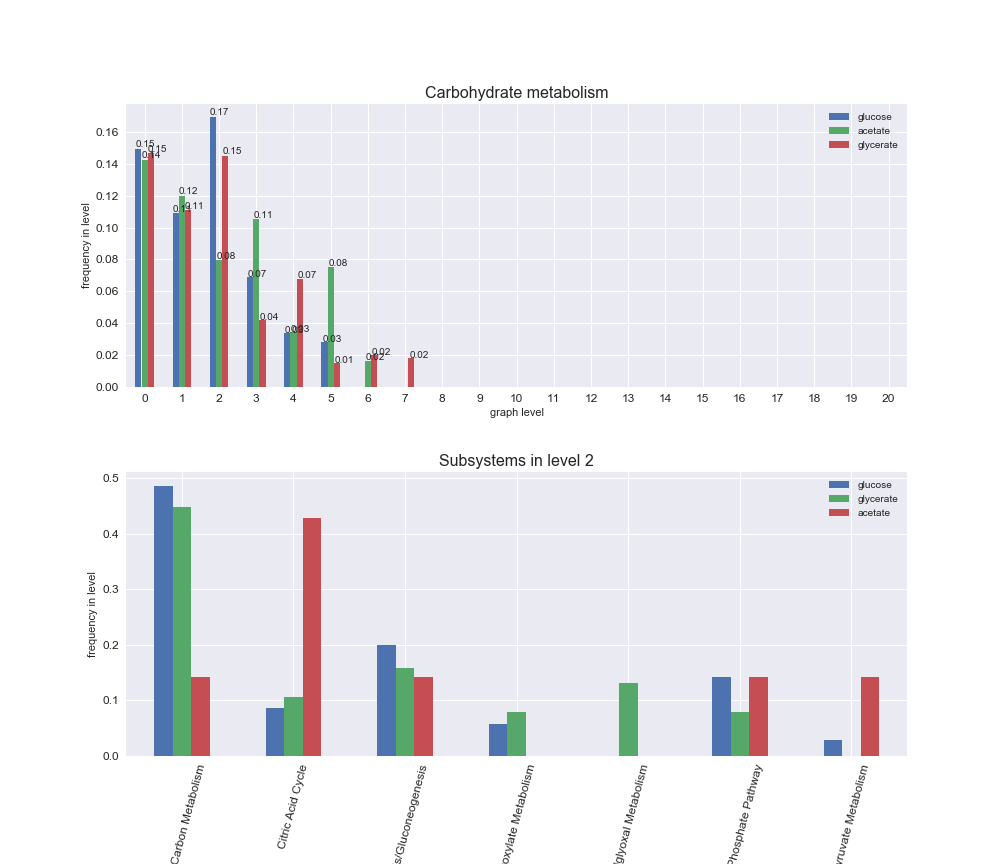
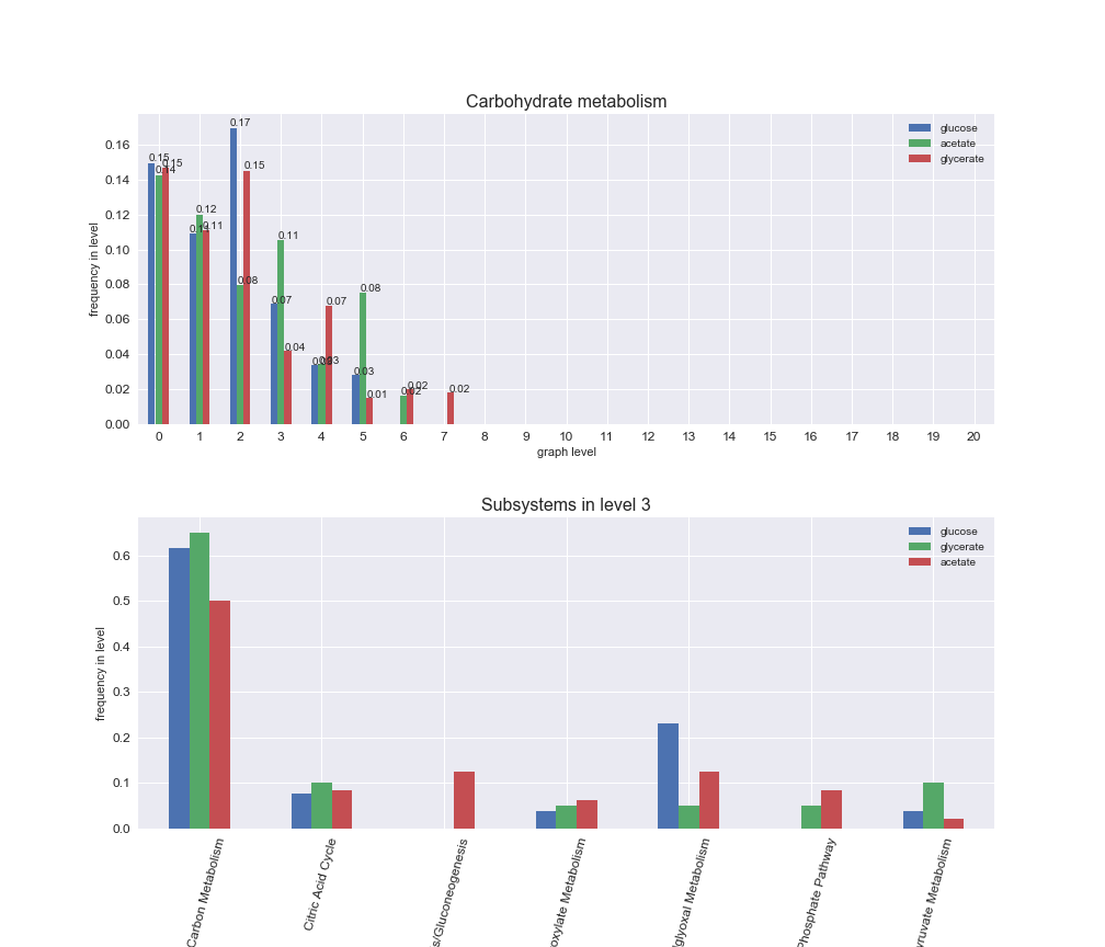
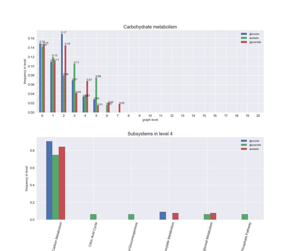
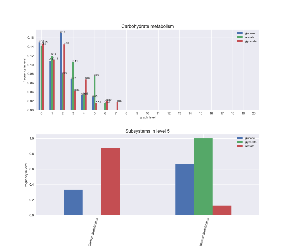
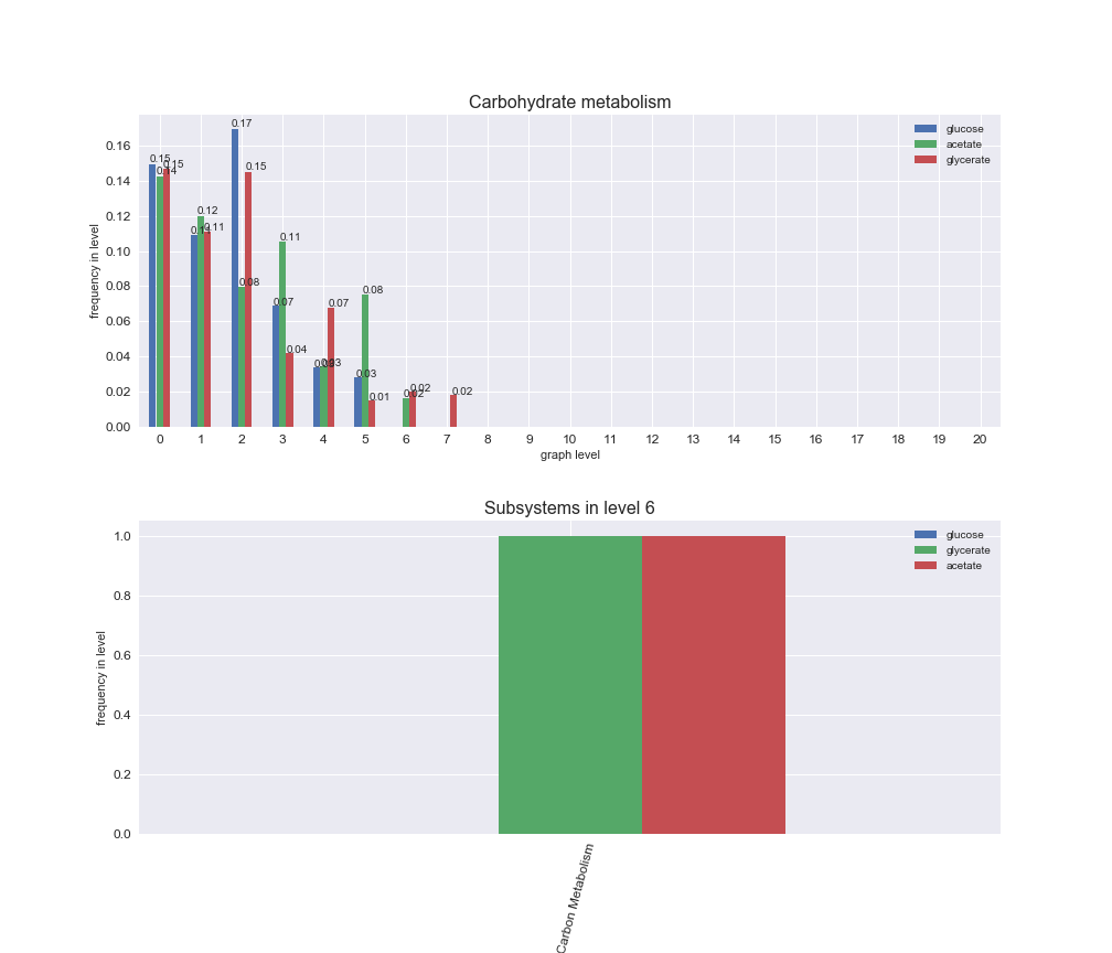
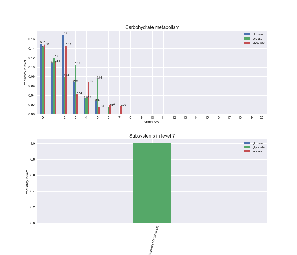


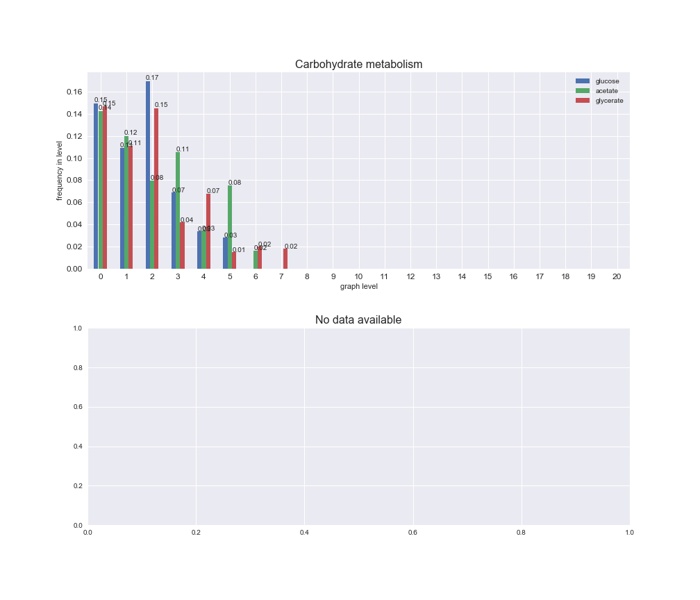


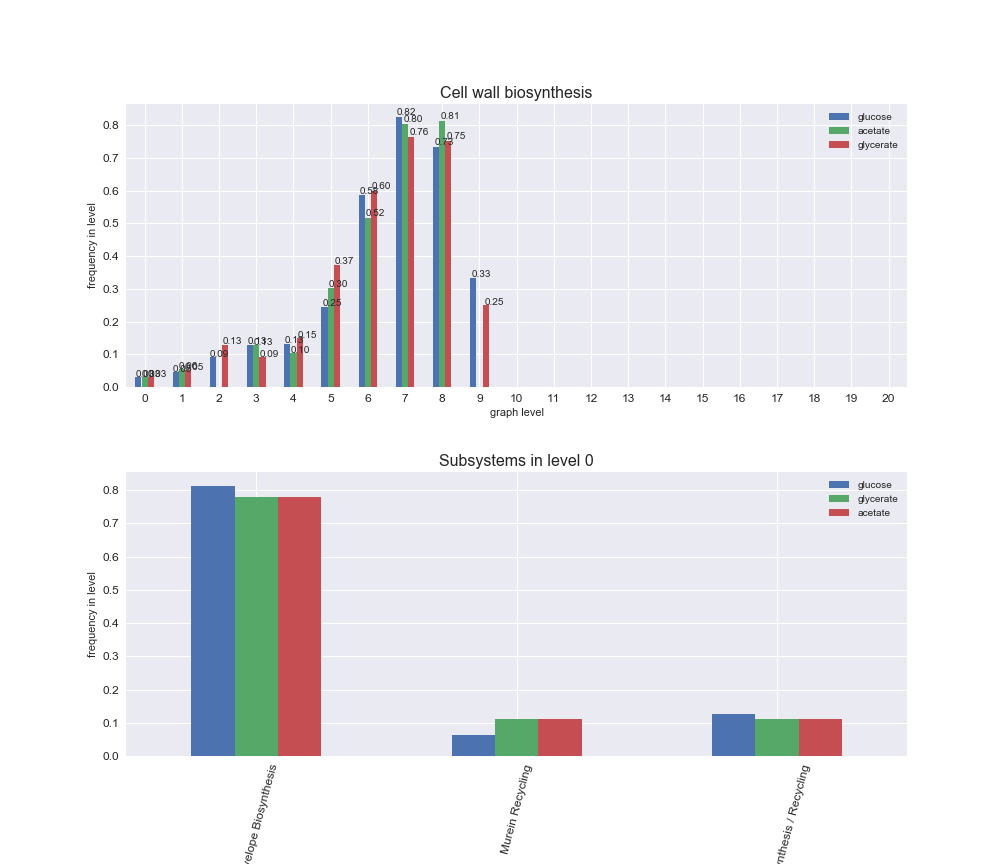
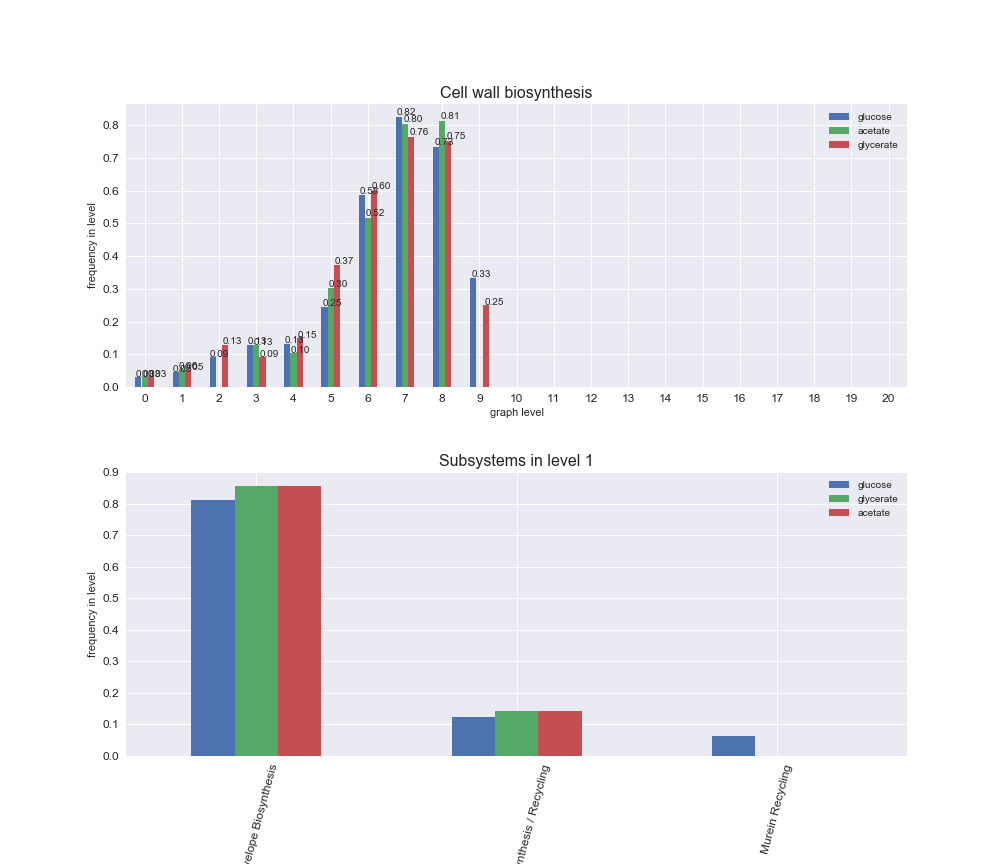
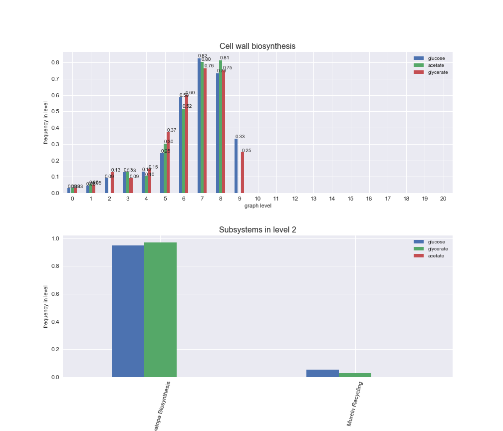
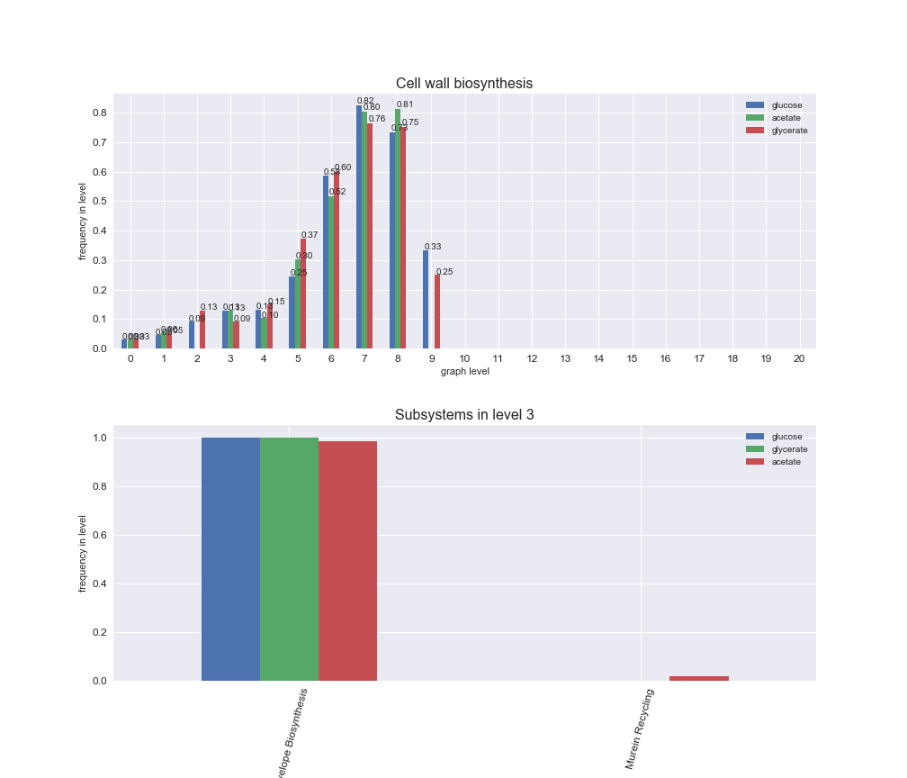
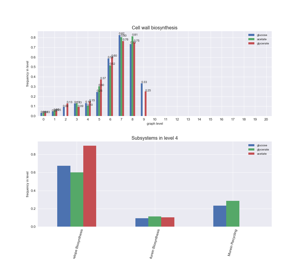
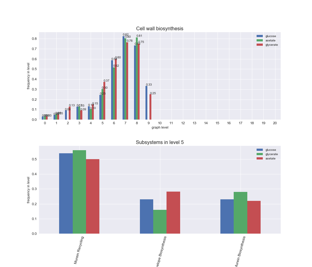
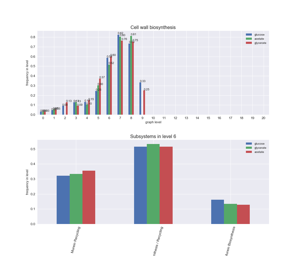
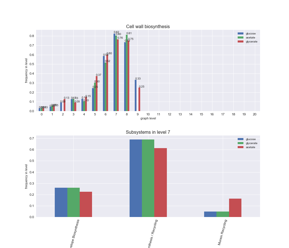
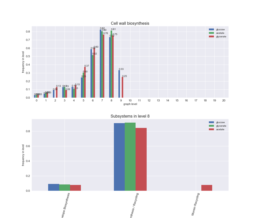
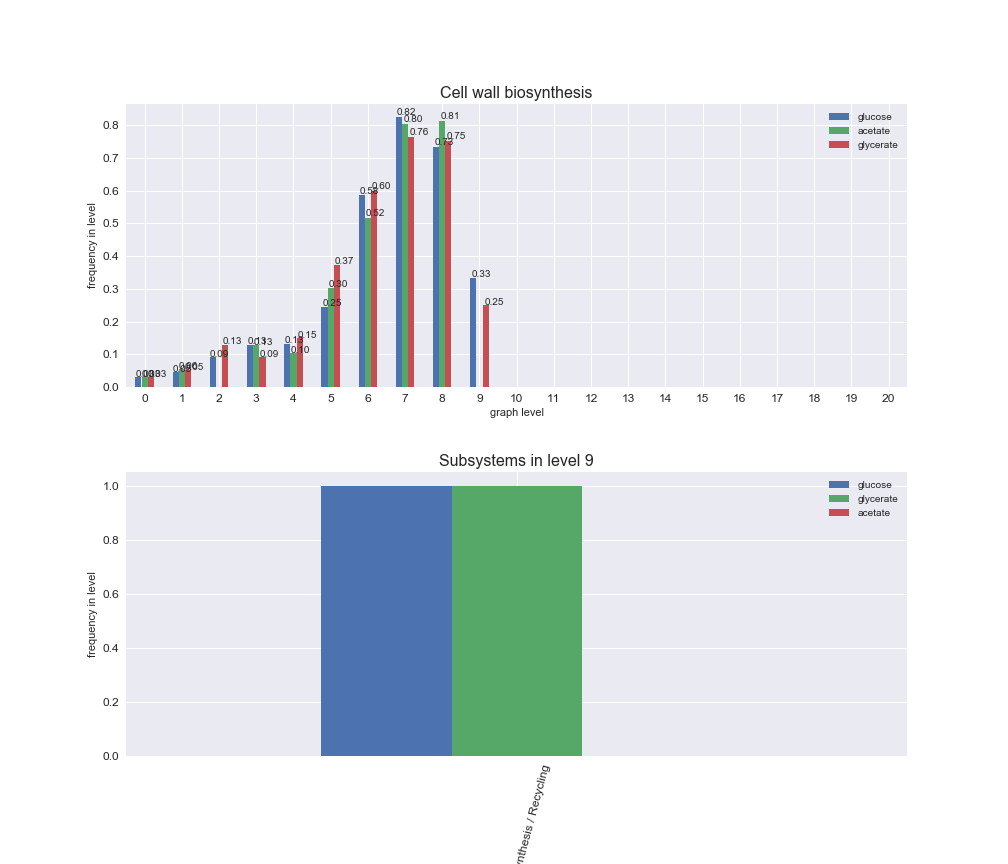


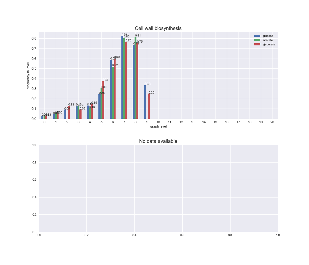


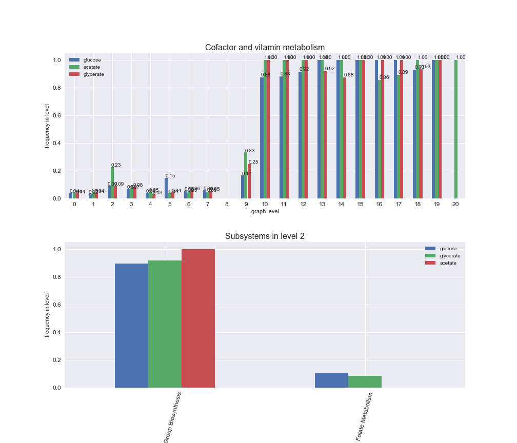


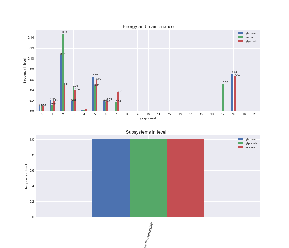
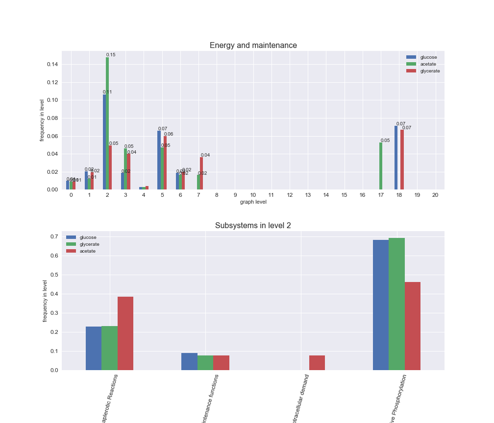
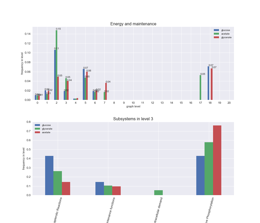

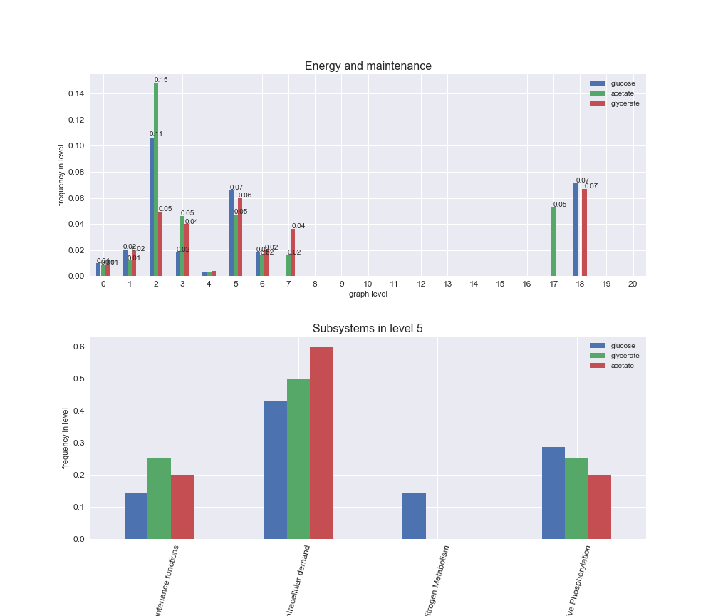
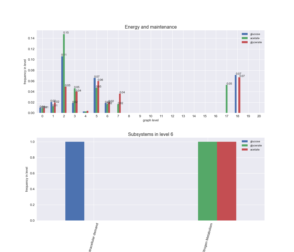
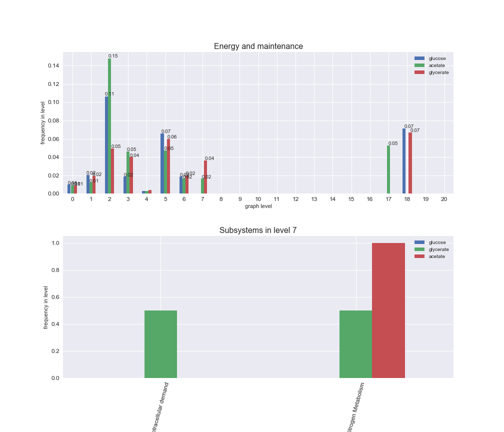
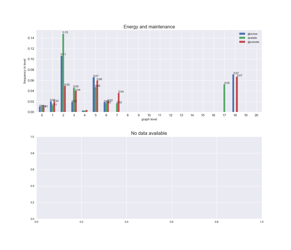


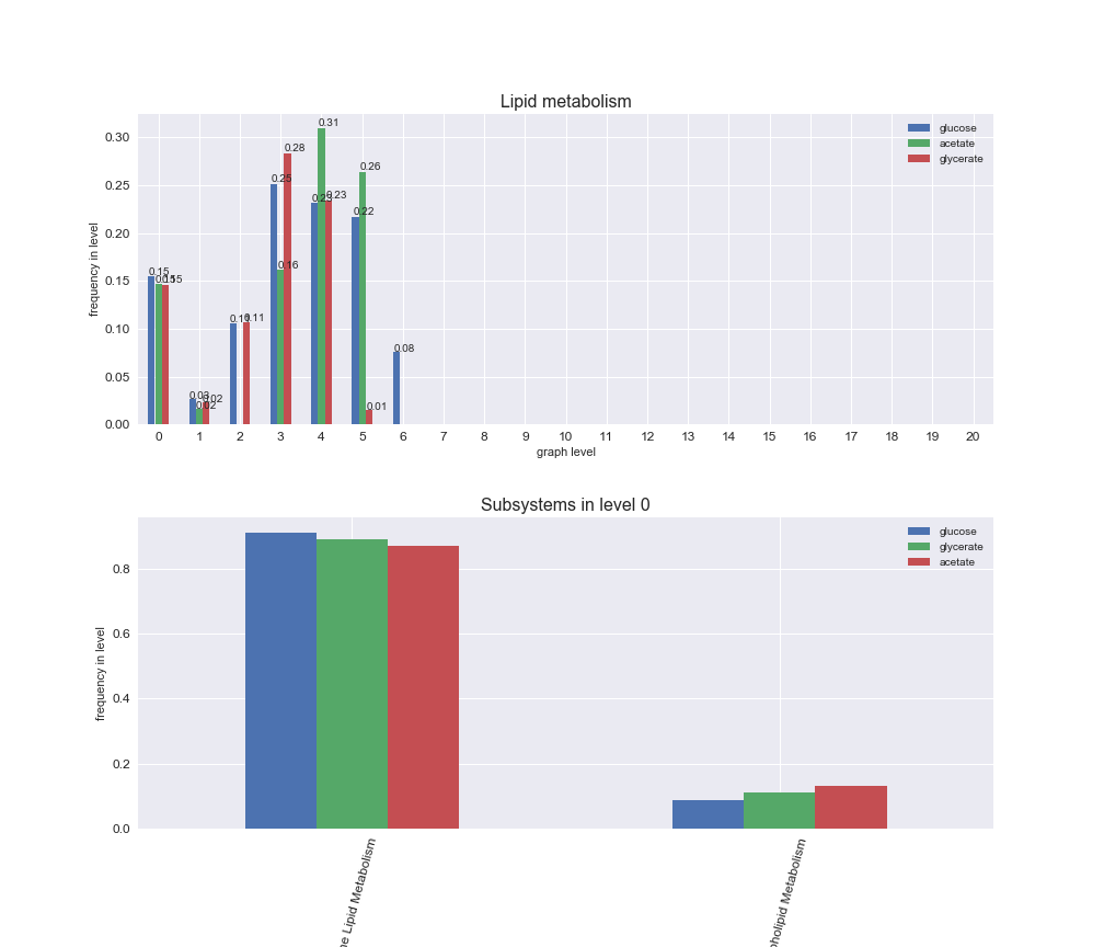
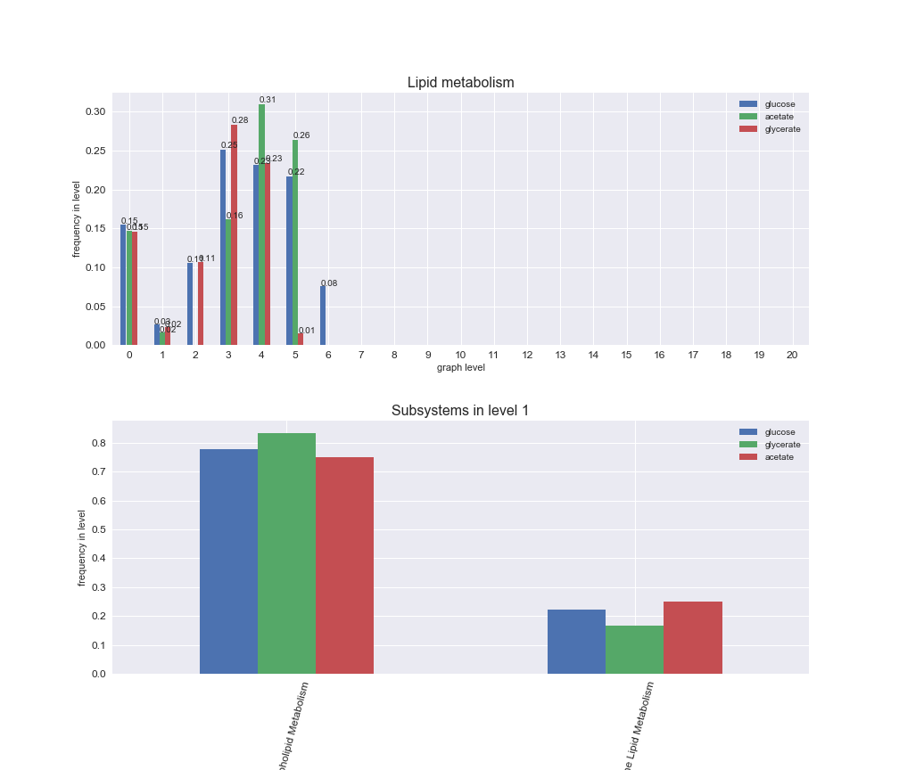
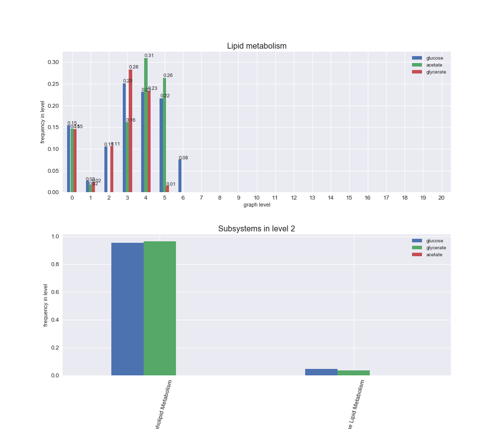
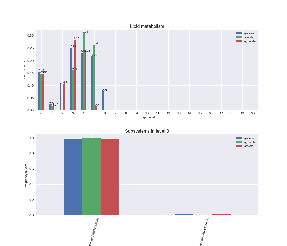
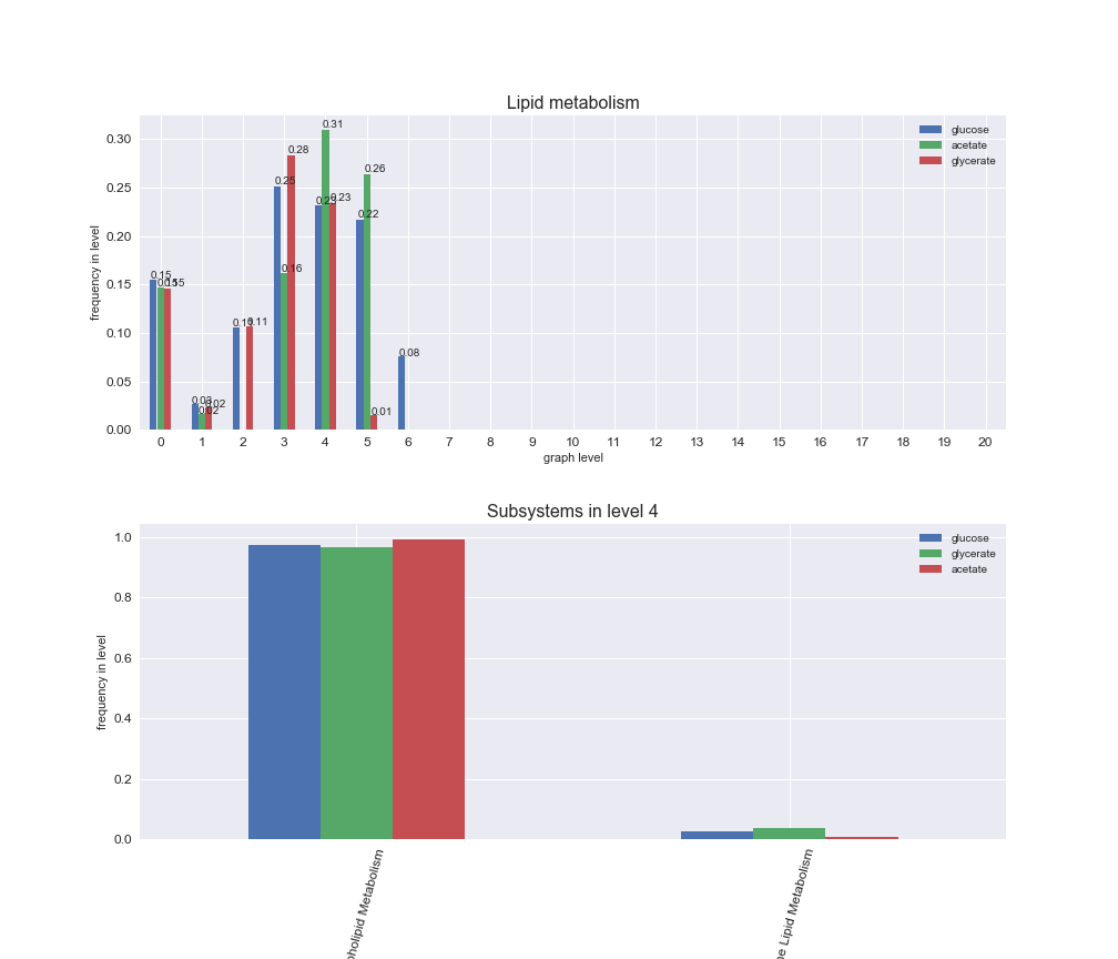
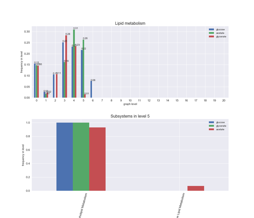
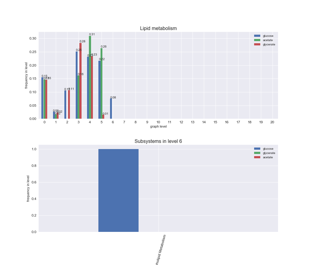


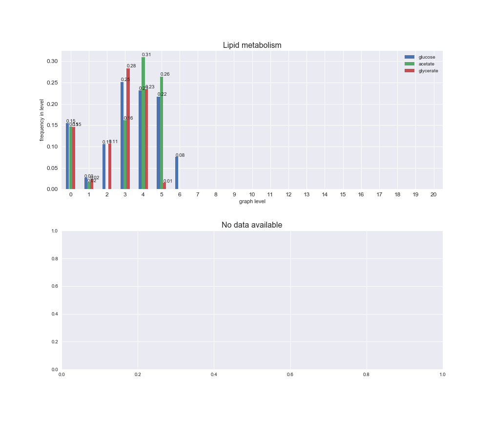


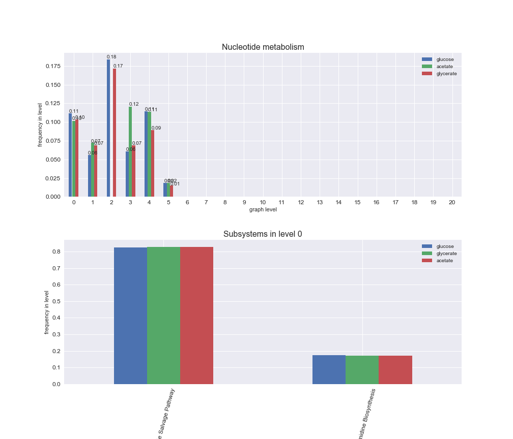
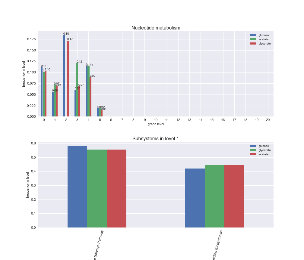
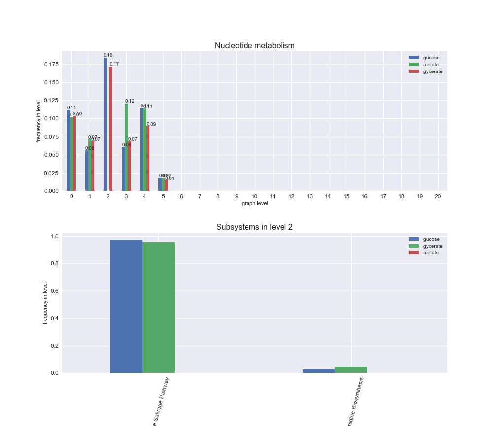
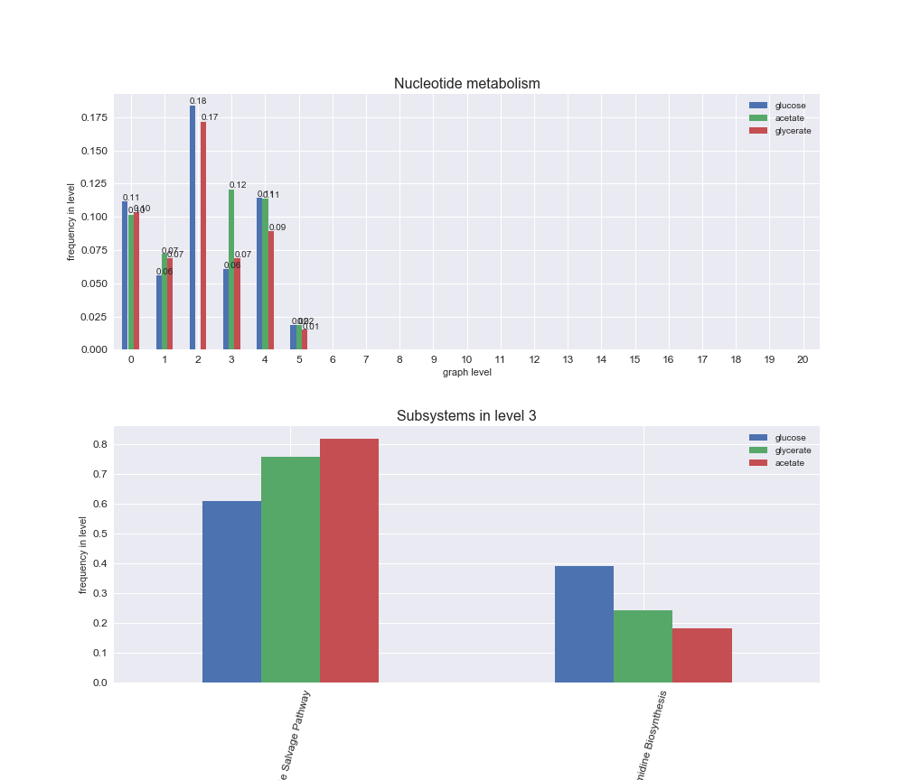
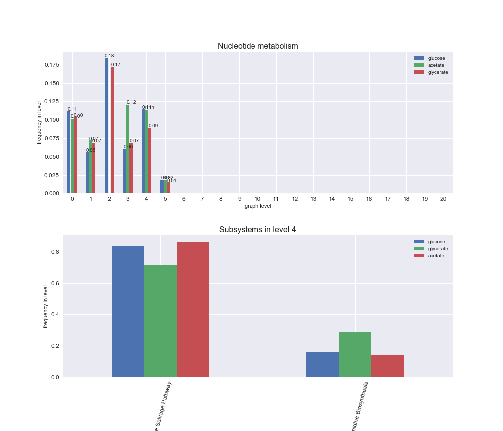
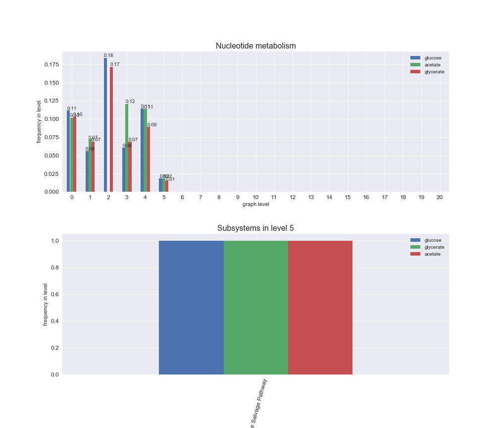

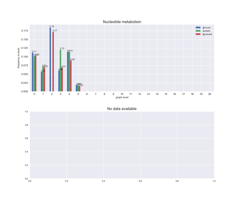


We see that the macrosystems are not uniformly represented across levels. Instead, each macrosystem is predominant in a particular region of the hierarchy. For instance, four macrosystems are only present within the first 8 levels: Nucleotide metabolism in the first 6 levels, Amino acid metabolism and Lipid metabolism in the first 7 levels and Carbohydrate metabolism in the first 8 levels. Additionally, while Cell wall biosynthesis is also only represented in the first 10 levels of the DAG, this macrosystem is predominant in levels 6 to 8, comprising between 52% and 82% of the reactions.
We can further increase the resolution and explore what subsystems are involved in some of the macrosystems observed previously. For instance, let's look at the picks found in levels 7-8 of Cell wall biosynthesis, in which over 73% of the reactions (across carbon sources) fall in this macrosystem. We see that in both level 7 and level 8, the majority of reactions are specifically in the subsystem Lipopolysaccharide Biosynthesis / Recycling.
3. The flux order relation in experimental data
In this section, we are going to test whether diverse data sets tend to follow the flux order relation previously described. We begin by collecting all required experimental data. Flux and transcript levels have been obtained from Ecomics an online database collecting data from multiple studies, while protein levels and $k_{cat}$ values have been obtained from . Finally, data on the total number of gene regulatory interactions, i.e., including both activating and inhibitory, have been obtained from the RegulonDB database . All data obtained corresponds to E. coli's K-12 strain, wild type and under no environmental stresses. Let's start by imported the data. For reproducibilty, all data files employed to generate the results presented in this notebook can be accessed from this DropBox repository.
# Parse experimental data
iJO1366_Data = DataParser(iJO1366['all'], workDir + '/Data')
proteinCosts = iJO1366_Data.getProteinCosts()
geneDataValues = {'transcript': iJO1366_Data.getTranscriptValues(),
                  'protein': iJO1366_Data.getProteinValues()}
fluxValues = iJO1366_Data.getFluxValues()
kcatValues = iJO1366_Data.getKcatValues()
geneRegulationData = iJO1366_Data.getGeneRegulatoryInteractions()

data_colors = {'transcript':'#ffbf00', 'protein':'#a217ed',
               'flux':'#25a9f4', 'kcat':'#b50636', 'activity':'#0acd47'}
costThresholds = [0, 70, 80, 85]
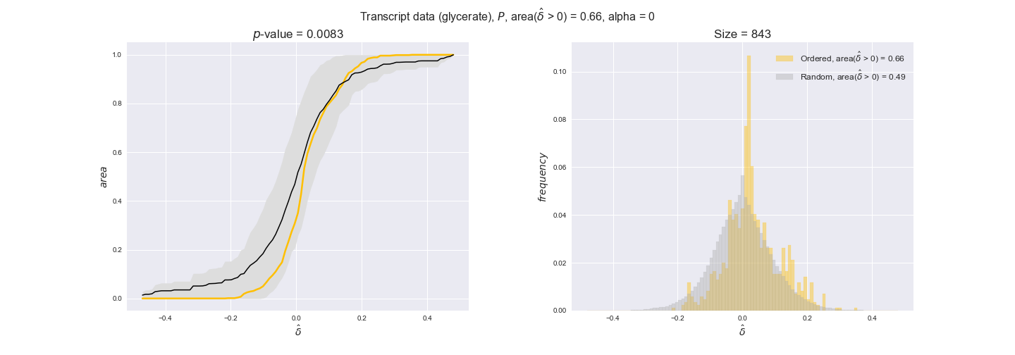
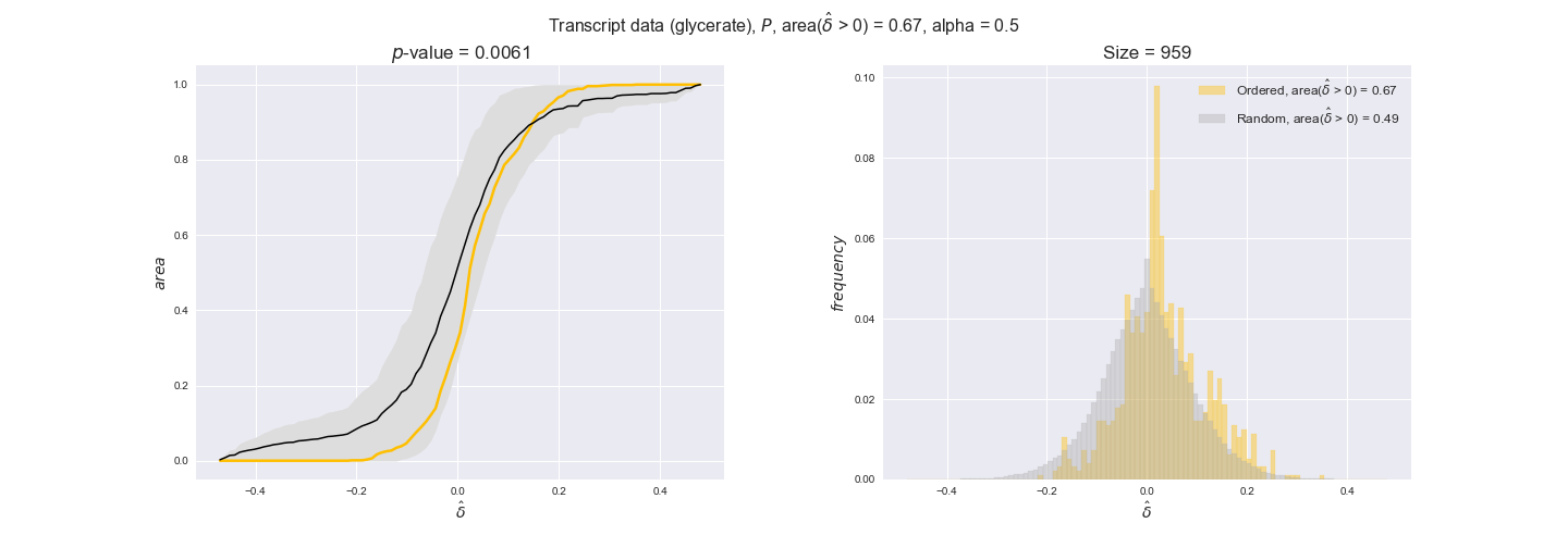
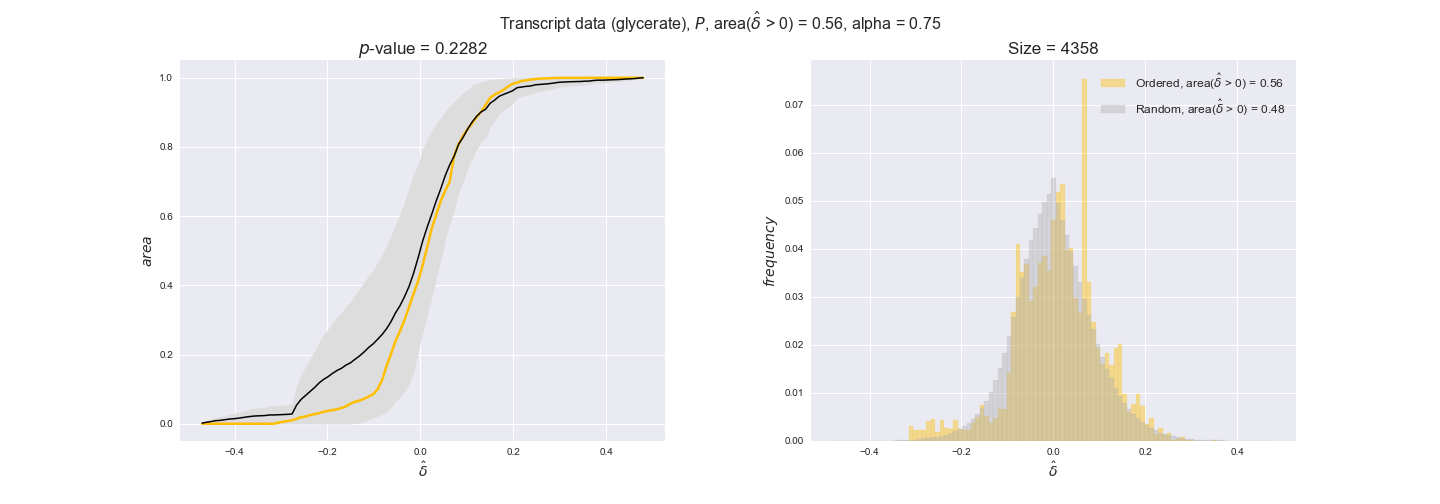
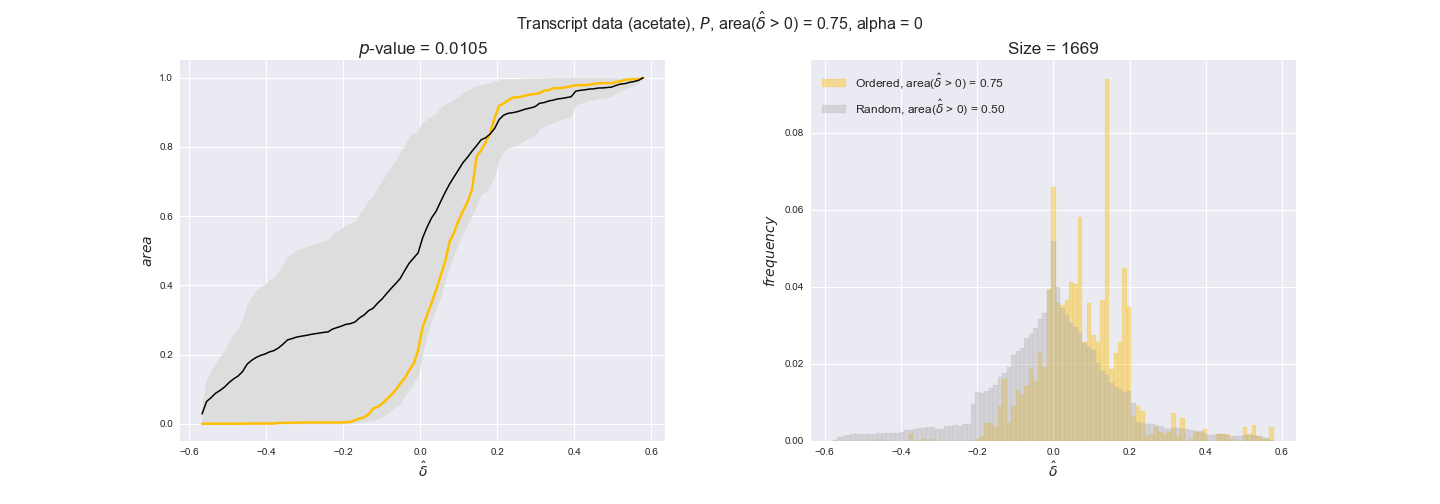
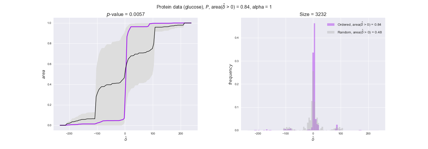
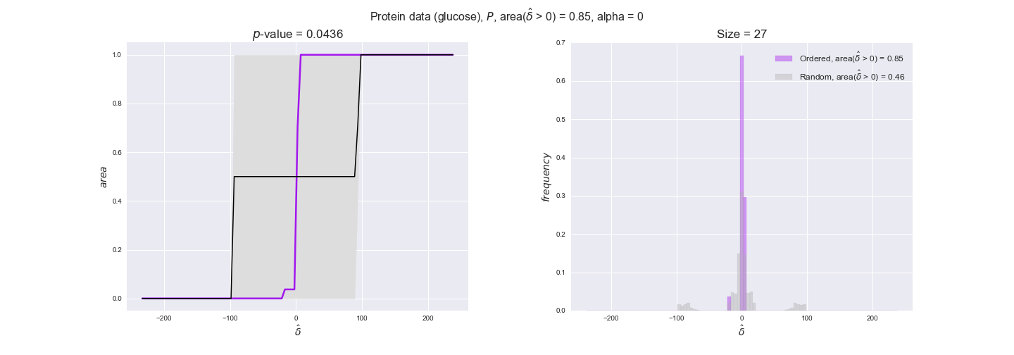
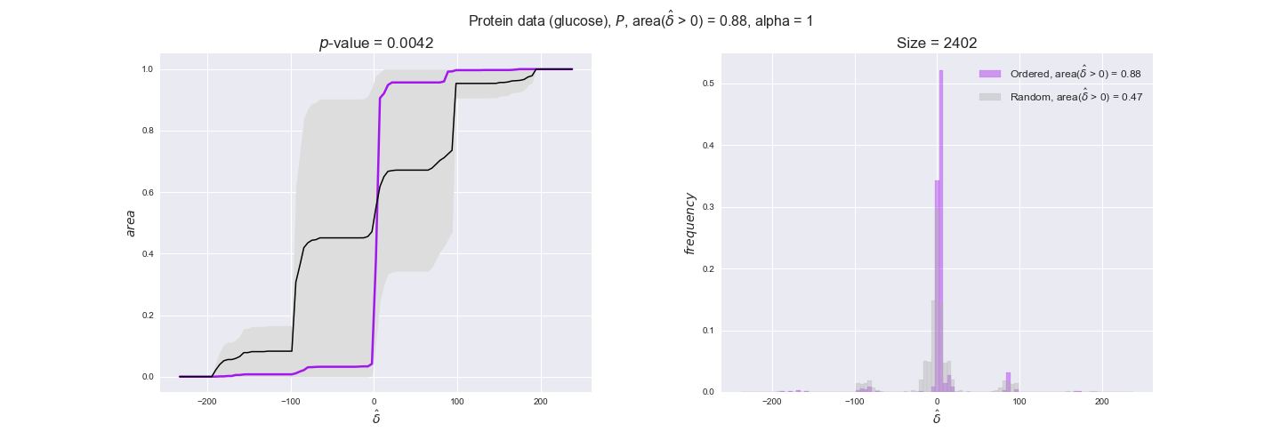
Now that we have all the data imported, we evaluate to what extent the flux order relation is respected by experimental data. We will do it in the following manner. First, we assign data to every reaction in the iJO1366 model — note that a reaction have multiple associated data values because of experimental replicates and more than one gene coding for the enzyme in the case of transcript and protein data. Next, for every pair of flux-ordered reactions, $r_i, r_j$, we compute the average difference in the assigned data values, i.e., $\hat{\delta_{ij}} = \hat{d_i} - \hat{d_j}$, where $\hat{d_i}, \hat{d_j}$ are the averages of the data assigned to the reactions. We know that $v_i \geq v_j$ thus $v_i - v_j \geq 0$, now we test to what extent $\hat{\delta_{ij}} \geq 0$ too. To this end, we compute the distribution of $\hat{\delta_{ij}}$ over all flux-ordered reaction pairs in the iJO1366 model, and take the fraction of positive values, i.e., $\mathrm{f}_{>0} = \Pr(\delta_{ij} > 0)$ as an indicator of the tendency of data to follow the flux order relation. Note that we use here positive values instead of nonnegative values. This is because we want to avoid the possible cases in which two reactions are assigned exactly the same set of data values, i.e., reactions catalyzed by enzymes that share all genes with available data, in which case $\hat{\delta_{ij}}$ would always be 0. Addtionally, we will perform a permutation test in which reactions are assigned random data drawn from the set of all avaialable data values. In this manner, we will have an idea of the significance of our observations. In this case, we have perform $n = 10000$ permutations and compute the experimental $p$-value = $(r + 1) / (n + 1)$, where $r$ is the number of samples $n$ with an equal or more extreme observation, hence the minimum $p$-value in this case is $10^{-4}$.
We will conduct the analysis for all carbon sources in case of transcript and protein data and only for glucose in the remaining datasets since these do not include the other carbon sources. Additionally, in the case of transcript and protein data, we will consider the metabolic costs associated to each reaction in the iJO1366 model. Specifically, we first associated a protein cost, i.e., moles of carbon source consumed per mole of protein synthesized, to each reaction in the model — protein cost data are obtained from . Next, we classify reactions in four groups based on the metabolic cost: i) all reactions in the model, ii) those with a cost which is larger than the percentile 70, $\mathrm{P}_{70}$, of the distribution of protein costs across all reactions, iii) those with a cost which is larger than $\mathrm{P}_{80}$ and iv) those with cost larger than $\mathrm{P}_{85}$. With this analysis, we will test whether transcript and protein levels tend to better follow the flux-order relation with increasing protein costs. An observation that would support the hypothesis that regulation of enzyme expression to match the flux-order relation (and hence avoid overproduction of unneeded enzymes) is more advantageous the higher the metabolic burden of synthesizing the enzymes.
Note that, so far, we have constrained the minimum flux through the biomass reaction to be 95% of the maximum possible, i.e., parameter $\alpha = 0.95$. However, it could be that the experimental data were taken under conditions in which _E. coli_ was growing at a larger or smaller rate. Therefore, we computed the flux-ordered reaction pairs for a range of $\alpha$ values from 0 to 1. The results are contained in the interactive figures. In some cases, results are not available for a particular $\alpha$ value. This is because no flux-ordered pairs with available data were generated under this particular value, e.g., only flux-ordered pairs generated with $\alpha \ge 0.95$ have flux data. In this notebook, we focus on describing the results obtained for $\alpha = 0.95$.
Let's go ahead and do the computation. Note, however, that performing the permutation test for transcript data and $n=10000$ can take a while (about 6 hrs with an Intel i5 CPU with 2.4 GHz). Results don't change much if a smaller sample, e.g. $n=500$, is drawn instead. Also, there is no need to run the code to see the results since the interactive figures work without a running kernel.
%%capture
# Get plot data for transcript and protein values
n_samples = 10000
int_plots_data = {'transcript': {}, 'protein': {}}
for data_type in int_plots_data.keys():
    for carbonSource in carbonSources:

        int_plots_data[data_type][carbonSource] = iJO1366_Orders[carbonSource].evaluateDataOrder(
            data=geneDataValues[data_type][carbonSource], proteinCosts=proteinCosts,
            costPercentileThresholds=costThresholds,
            samplesizen_samples)

# Get plot data for flux, kcat and activity values
flux_plot_data = iJO1366_Orders['glucose'].evaluateDataOrder(
    data=fluxValues, samplesize=n_samples)
# kcat values are independent of carbon source, for this
# reason, we test them in all carbon sources
kcat_plot_data = {}
for carbonSource in carbonSources:
    kcat_plot_data[carbonSource] = iJO1366_Orders[carbonSource].evaluateDataOrder(
    data=kcatValues, samplesize=n_samples)
3.1. Flux levels and the flux order relation
Let's plot the histogram and cumulative distribution of average data differences obtained from flux level data. In both plots, results generated with the actual (unpermuted) data are depicted in blue while those coming from the permutation analysis are depicted in gray. Additionally, we plot the range covered by all $n=10000$ cumulative distributions generated in the permutation analysis (gray-shaded region in the left plot) as well as the cumulative distribution corresponding to the sum of all $n$ distributions of (permuted) data differences, depicted in black in the left plot — the sum of all $n$ distributions generated in the permutation is depicted in gray in the plot on the right.
flux_plot = pm.plotDataOrder(flux_plot_data, data_colors['flux'], interactive=True, has_protein_costs=False)
flux_plot
alpha (biomass):
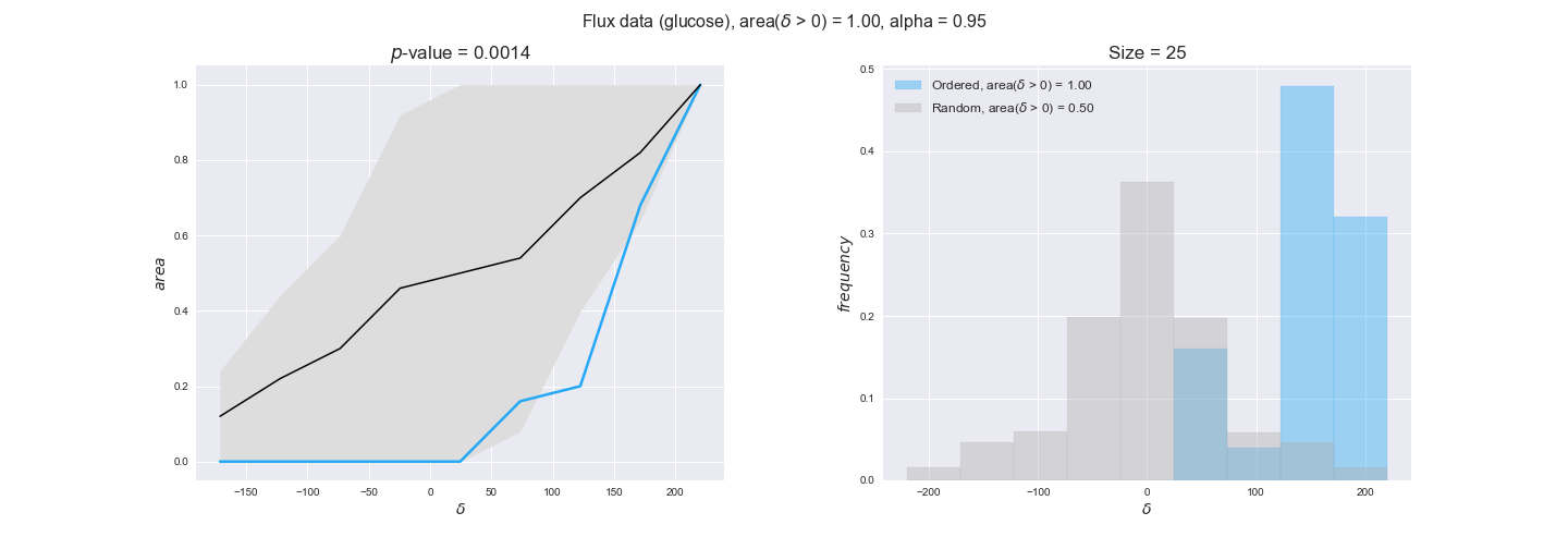
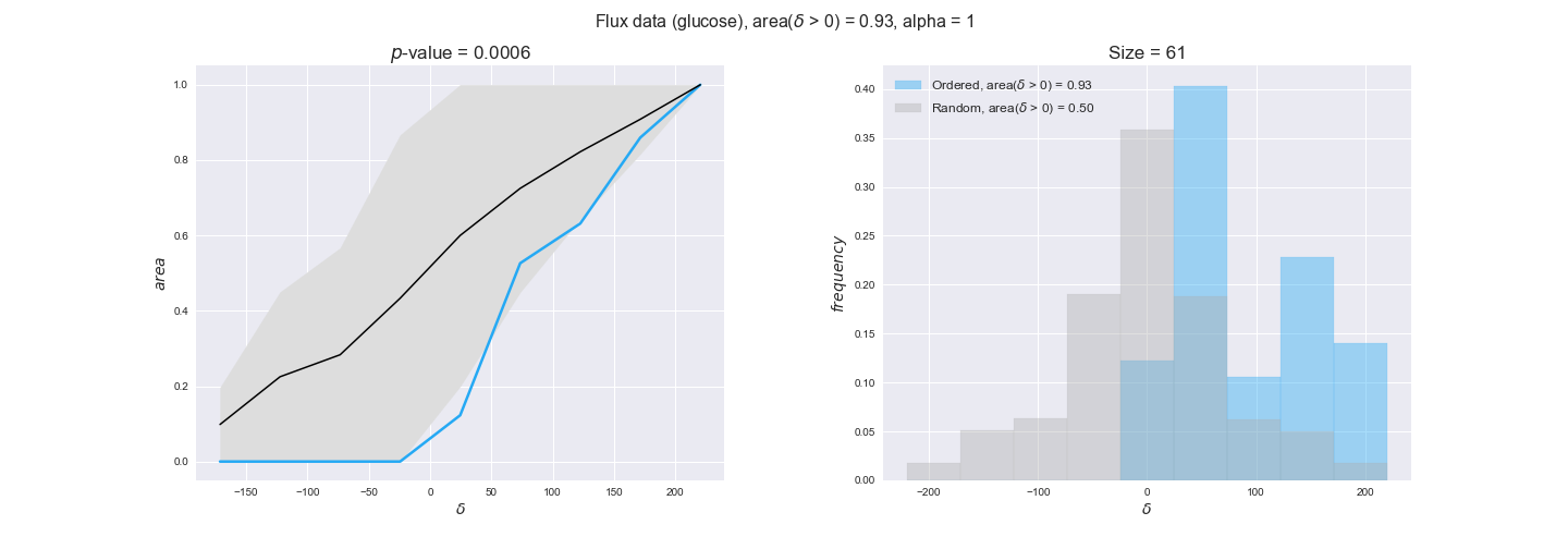
We see that flux data satisfy the flux order relation in all cases, i.e., in all 25 flux-ordered pairs with available data, the difference of reaction flux levels is always positive. Moreover, the low $p$-value = 0.0015 indicates that these results are likely to be significant. This result is in line with what we would expect since flux level data is the only data type directly comparable to our prediction on the ordering of fluxes.
While the previous was a very good result, it could be an artifact. Estimating flux levels from ${}^{13}\mathrm{C}$ measurements requires a metabolic network. The largest part of the flux data used in this study comes from , in which authors employed a small metabolic network, covering the central carbon metabolism, to calculate the flux levels that better explained the ${}^{13}\mathrm{C}$ measurements. It could be possible that the small metabolic network, here termed experimental network, produced a set of flux-ordered reaction pairs that was also within the set of flux-ordered pairs of iJO1366. If this were to be the case, then the order relation observed in the flux level data would be a necessary consequence of the method employed to obtain the data and not a reflection of the order relation in iJO1366. To investivate this issue, we will find the flux-ordered pairs of the experimental network and evaluate if they are in fact within the set of flux-ordered pairs of iJO1366. Let's start by importing the experimental network which was obtained from supplementary Sfigure2 of the above publication and computing the flux-ordered pairs here.
FluxDataNetwork = pd.read_excel(workDir + '/Models/FluxDataNetwork/FluxDataNetwork.xlsx', header=4, index_col=0)
n_mets_exp, n_rxns_exp = FluxDataNetwork.shape
print('Experimental network imported with {} reactions and {} metabolites'.format(n_rxns_exp, n_mets_exp))
Let's continue and compute the flux-ordered reaction pairs of the experimental network. This metabolic network was directly obtained from an excel file instead of being part of a cobra model. For this reason, we will use a dedicated function to find flux-ordered pairs in this case instead of using the class Model as before.
FluxDataNetwork_Orders_DataFrame = hm.getFluxOrdersForFluxDataNetwork(
    FluxDataNetwork, carbonUptakeRate=20, fva_filter=True)
We see that indeed the experimental network is capable of generating flux-ordered reaction pairs, a total of 92 (6.4%) pairs. Next, we look at the intersection between this set and the set of flux-ordered pairs of iJO1366.
iJO1366_Orders_DataFrame = hm.getFluxOrderDataFrame(iJO1366_A['glucose'], iJO1366['glucose'])
shared_ordered_pairs = hm.getSharedOrderedPairs(
    FluxDataNetwork_Orders_DataFrame, iJO1366_Orders_DataFrame, reactionsWithData=fluxValues.keys())

shared_ordered_pairs['total']
We see that 8 out of the 92 pairs in the experimental network are shared with iJO1366. However, we only care about the pairs for which experimental data are available. If we consider only those with available flux levels the list reduces to 5 reaction pairs:
shared_ordered_pairs['with data']
That is, a proportion of $1/5$ of the 25 flux-ordered pairs with flux data evaluated before are shared between models and hence the ordering of data values can be considered an artifact in $1/5$ of the cases. Therefore in the majority of cases, flux levels were respecting flux-ordered pairs that were genuine to JO1366. Finally, let's make sure that flux level data follow, as it must, the flux order relation in the experimental network. We will use the same method employed in the iJO1366 model.
flux_plot_data_ExpNet = DataOrderEvaluator(
    FluxDataNetwork_Orders_DataFrame, data=fluxValues).evaluateDataOrderRelation(samplesize=10000)
flux_plot_ExpNet = pm.plotDataOrder(
    flux_plot_data_ExpNet, data_colors['flux'], interactive=False)

Once again, we see that flux levels respect the flux order relation in all cases, i.e., 22 flux-ordered pairs with available data in the experimental network. Furthermore, the obtained experimental $p$-value indicates that this result is solid. We conclude that flux levels do entirely respect the flux order relation. Next, we will investigate to what extent this result holds when using other, indirect measurements of reaction rate
3.2. Transcript and protein levels and the flux order relation
Here, we conduct the same analysis that we performed in the previous section. However, this time we will use transcript and protein levels. These data types differ from flux levels in two ways. On the one hand, these are indirect measurements of flux rate, at best we can hope for some correlation between transcript and protein levels and flux levels. This is because reaction flux not only depends on the amount of enzyme (even less on the amount of gene transcripts) that is available. Specifically, reaction flux is a rather complicated function of the amount of active enzyme catalytic centers — including the possibility here of enzyme regulation — enzyme catalytic rate and metabolite concentrations. On the other hand, we have a markedly larger set of data values for each reaction and a greater coverage since i) enzymes can be coded by more than one gene and ii) current technology makes it easier and more accessible to measure transcript and protein levels than flux levels and it is not limited to reactions in central carbon metabolism. Let's then continue our analysis evaluating the flux-order relation in transcript data. Remember that in both, transcript and protein data, we will consider the three carbon sources as well as the metabolic cost required to synthesize enzymes. Consequently, we generate a total of 12 plots — three carbon sources and four cost thresholds for each carbon source.
transcript_plots = pm.plotDataOrder(transcript_plot_data, data_colors['transcript'], interactive=True)
transcript_plots
Percentile:
alpha (biomass):
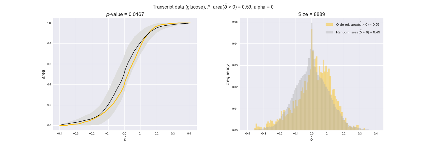
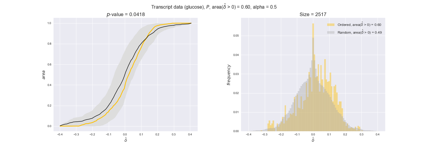
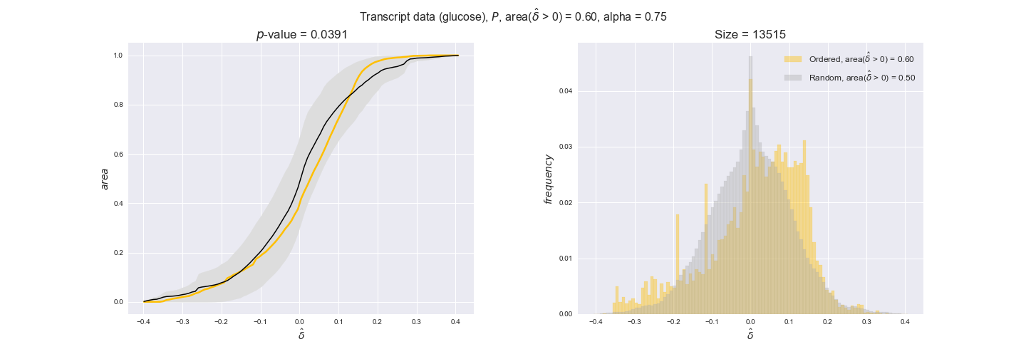

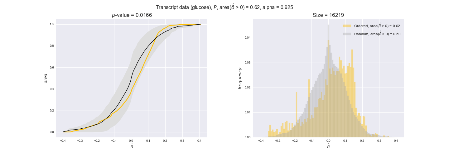
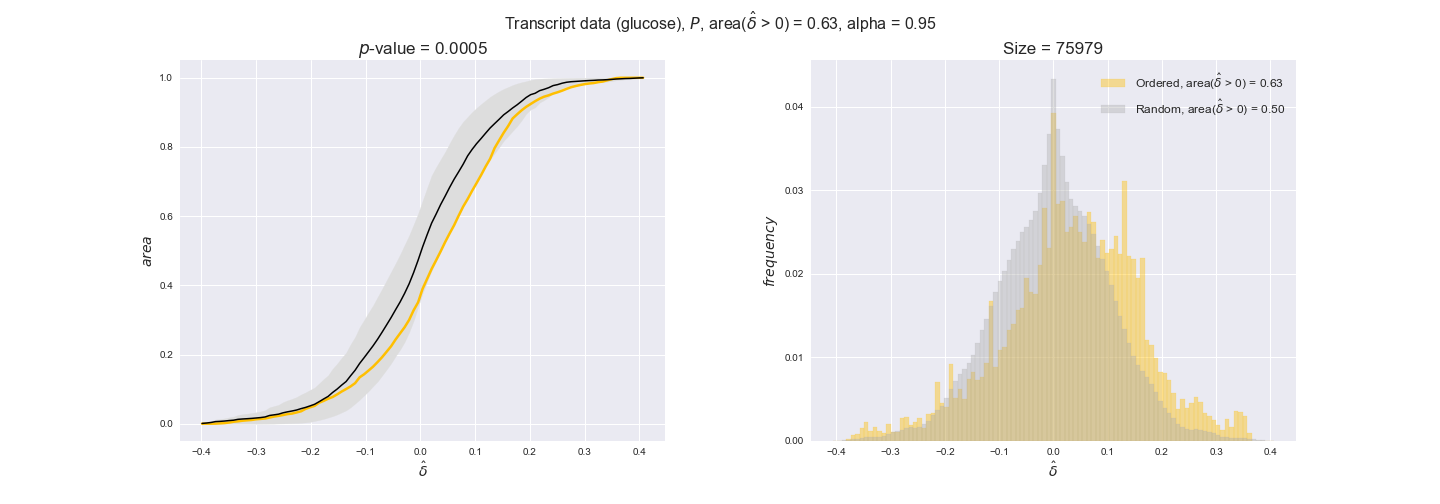
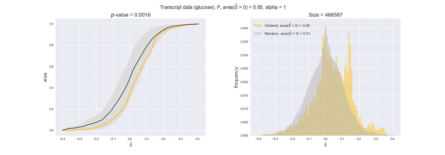
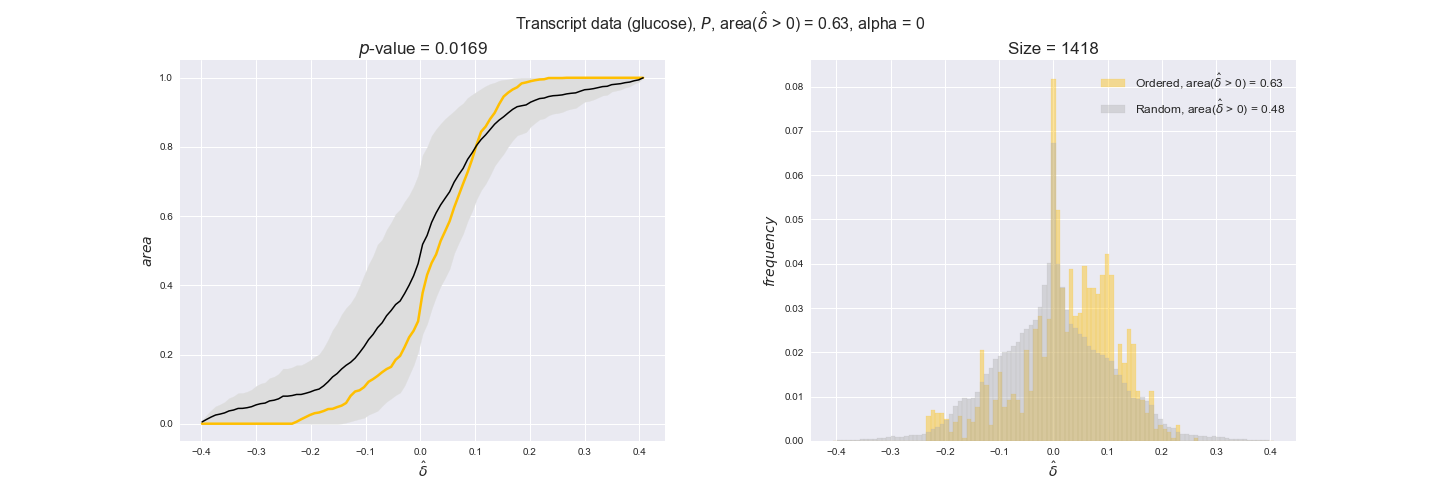

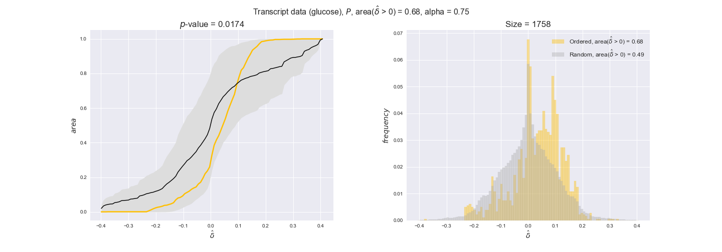
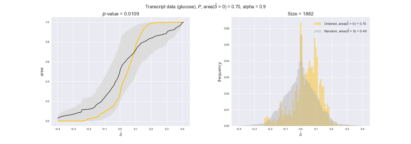
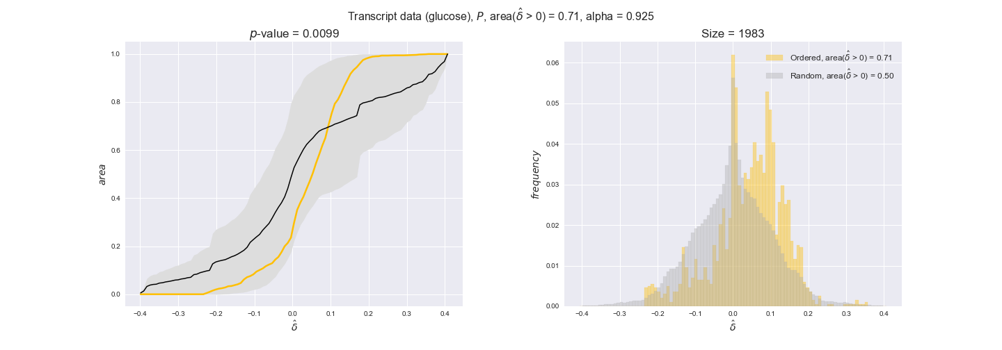
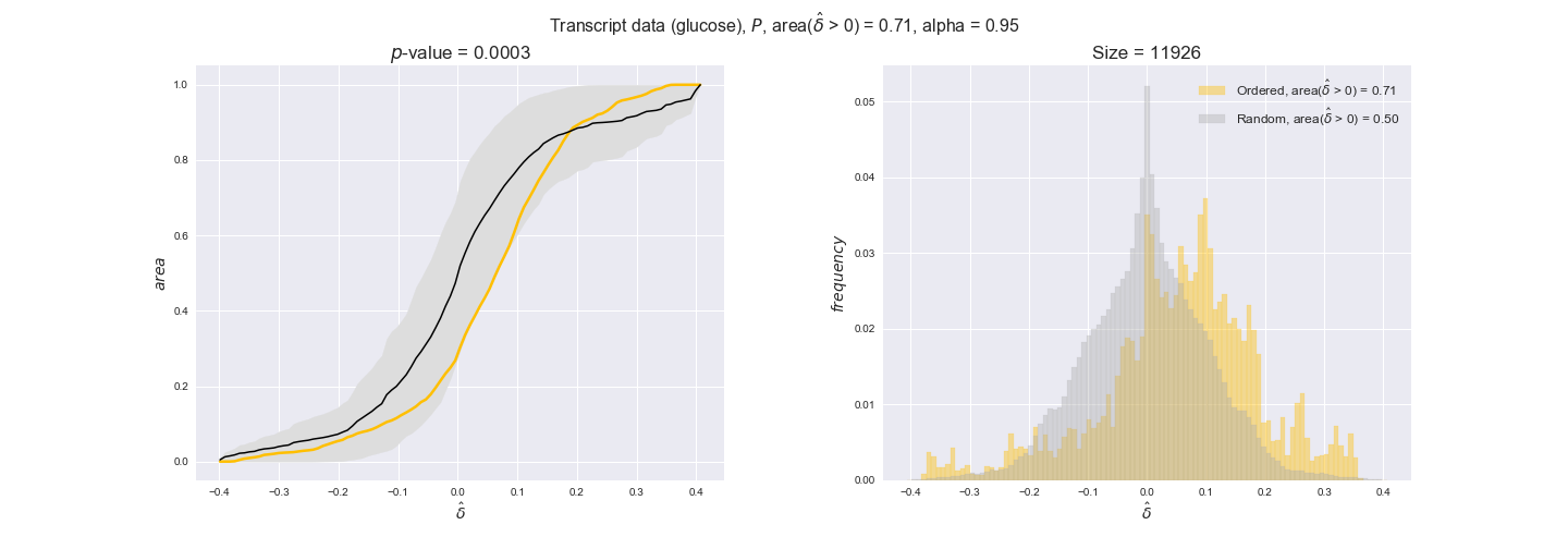
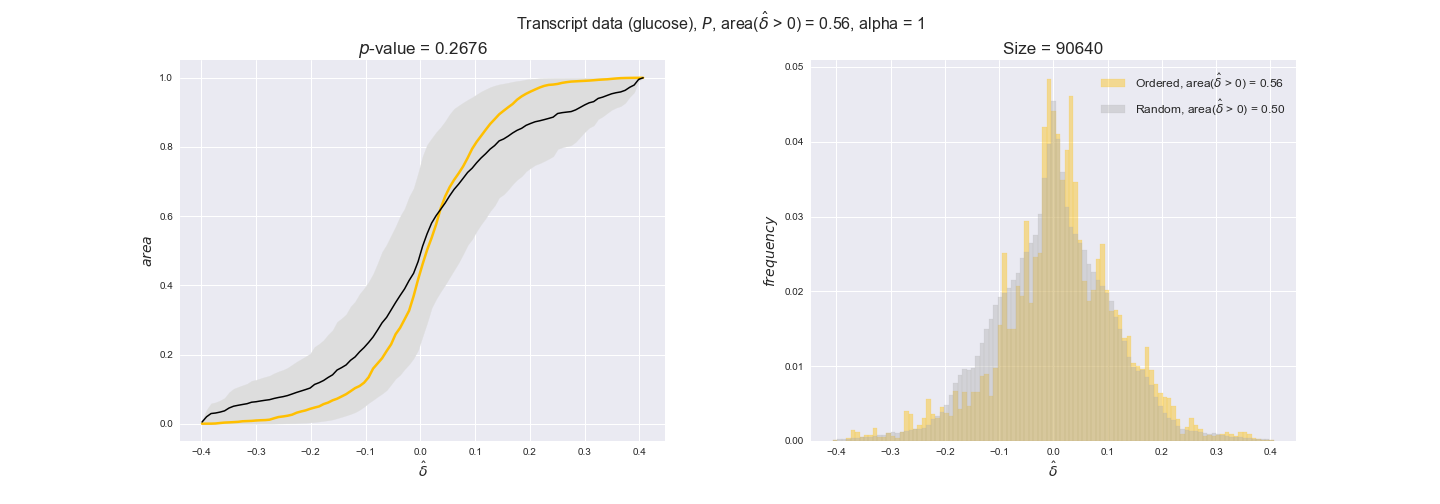
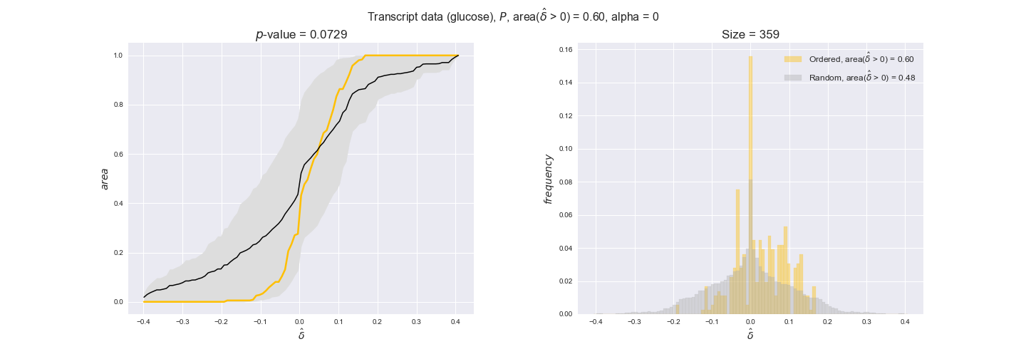
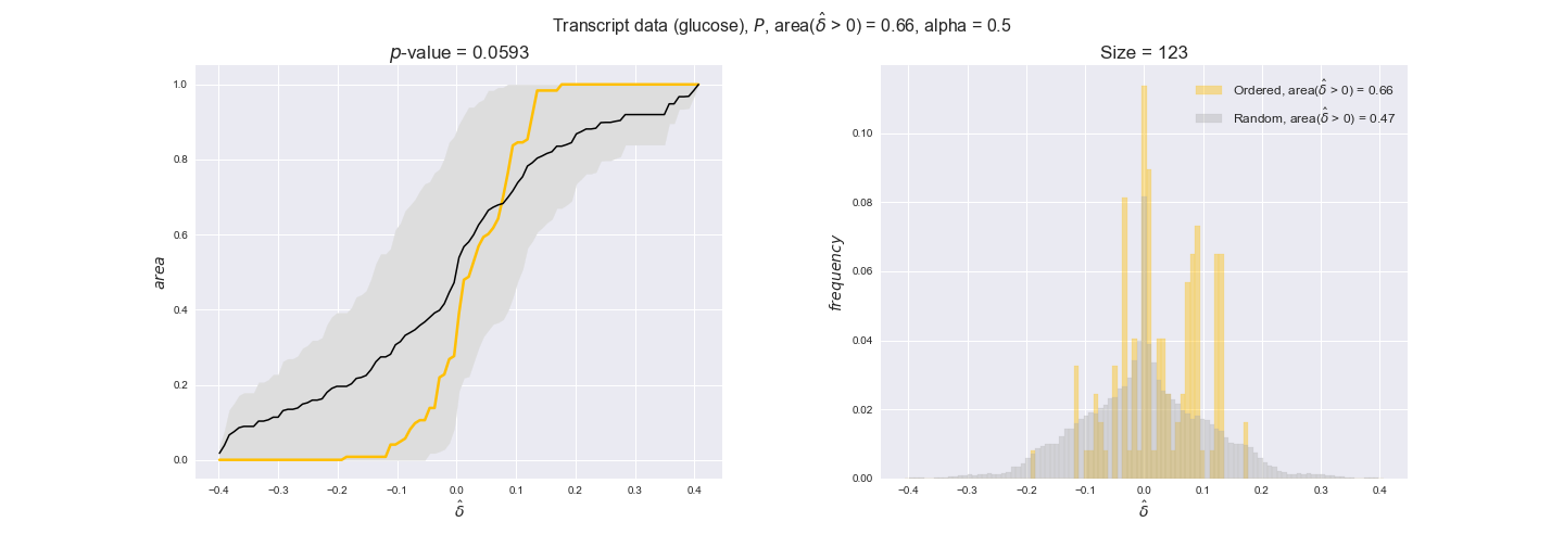
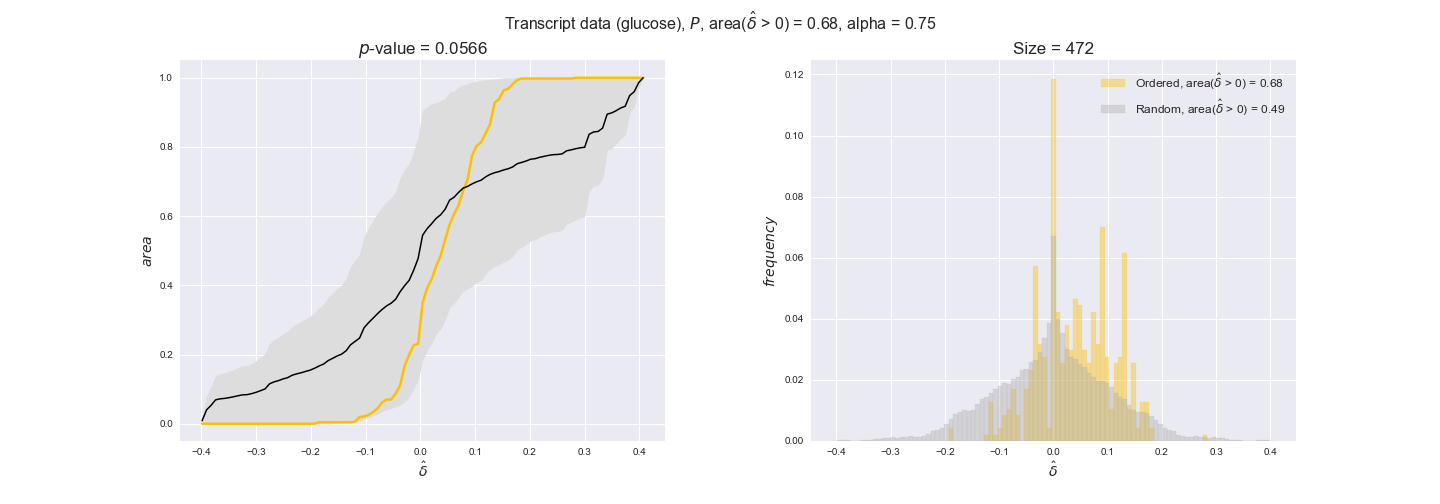
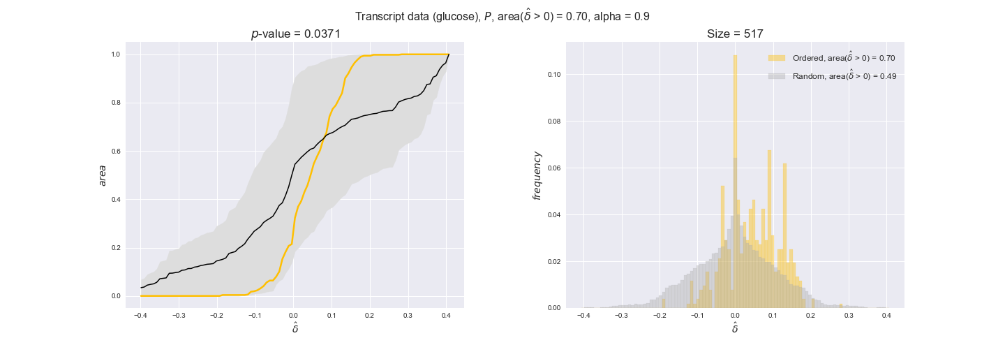
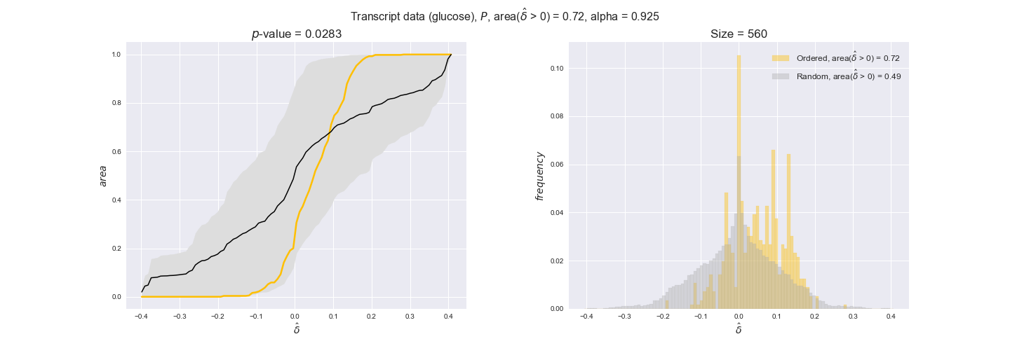

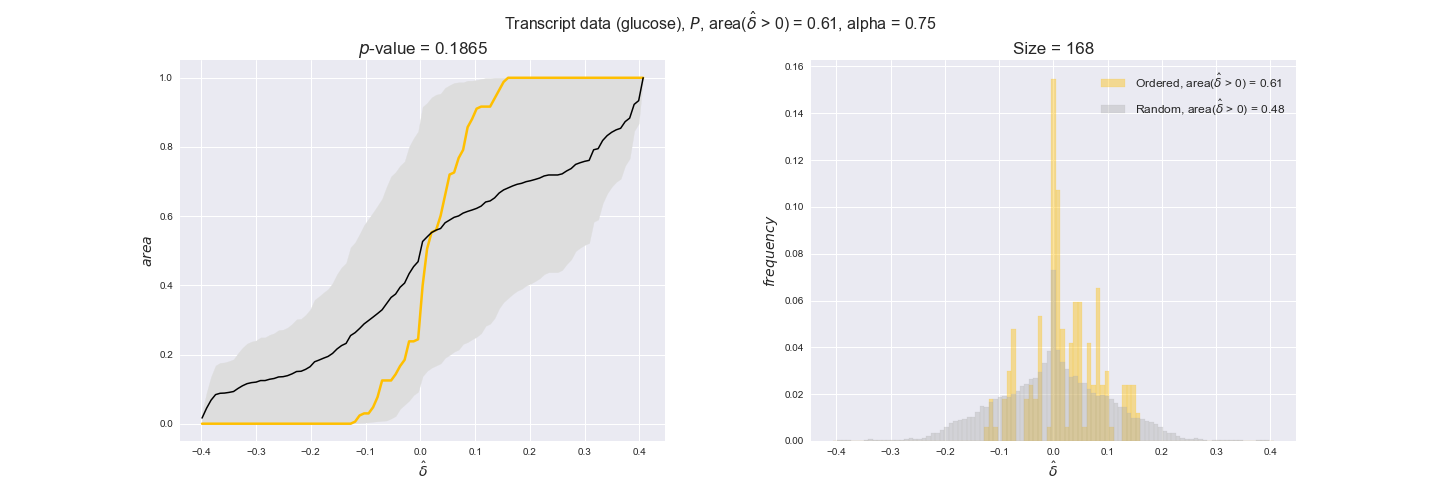
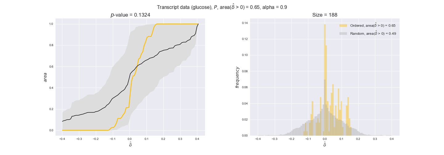
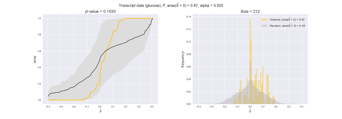
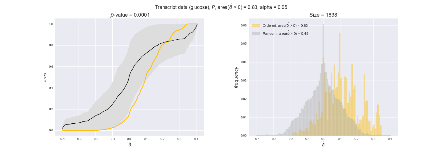
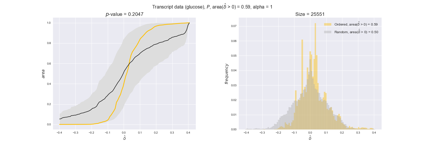
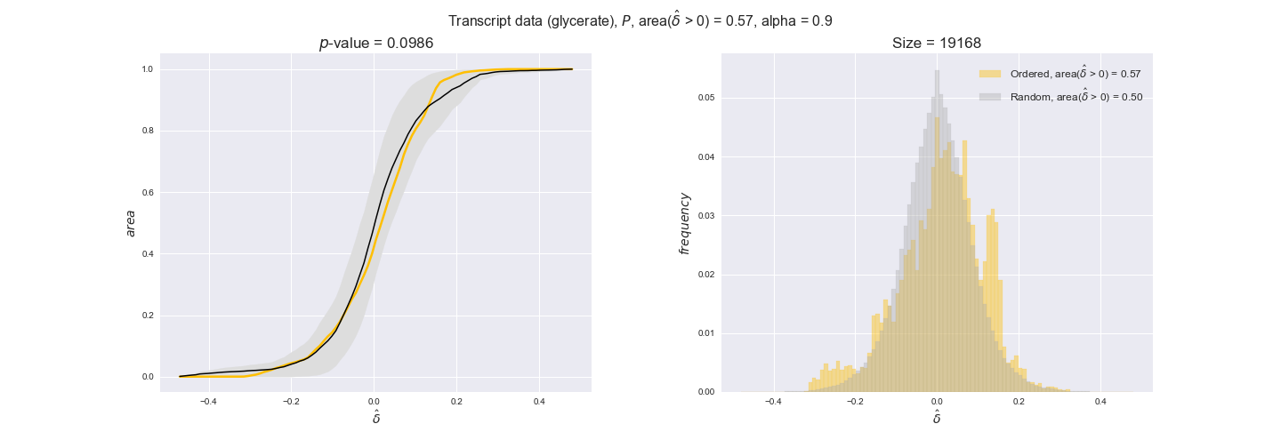
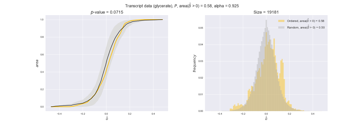
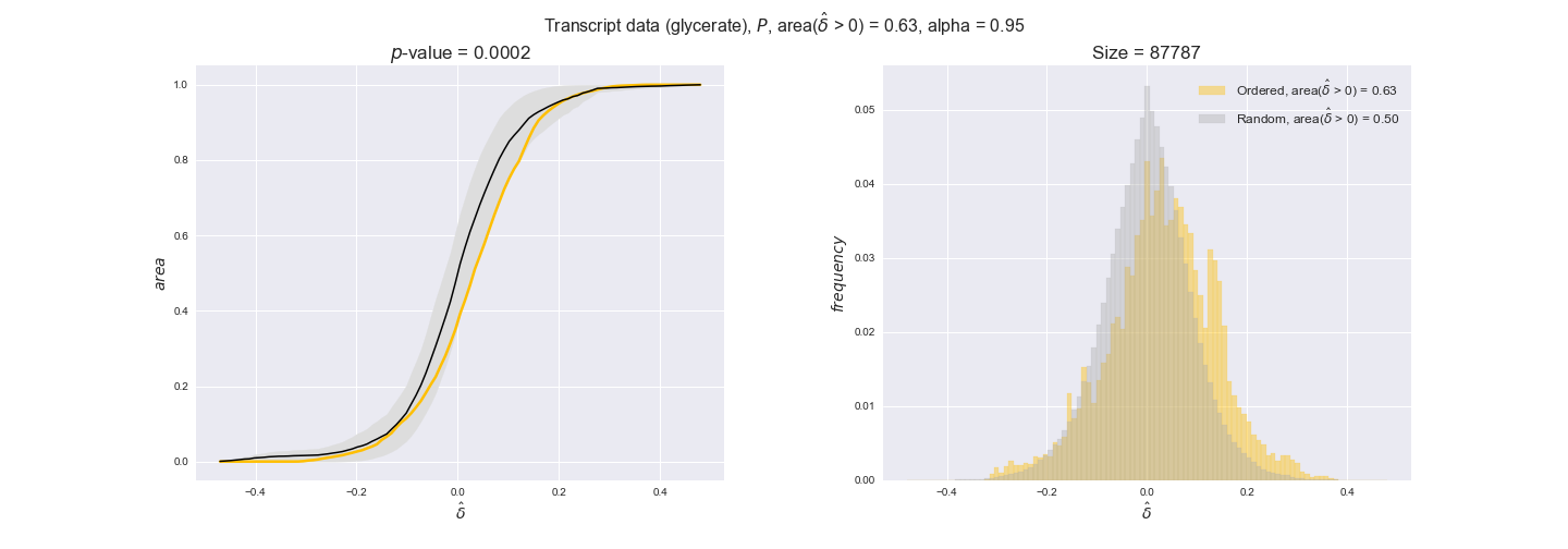


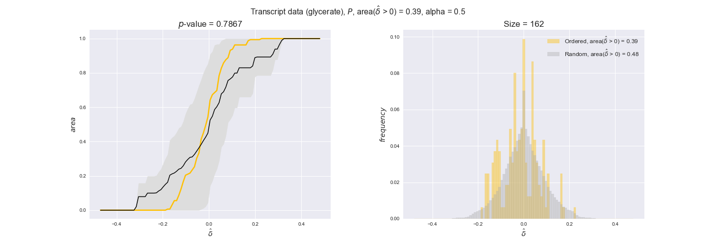
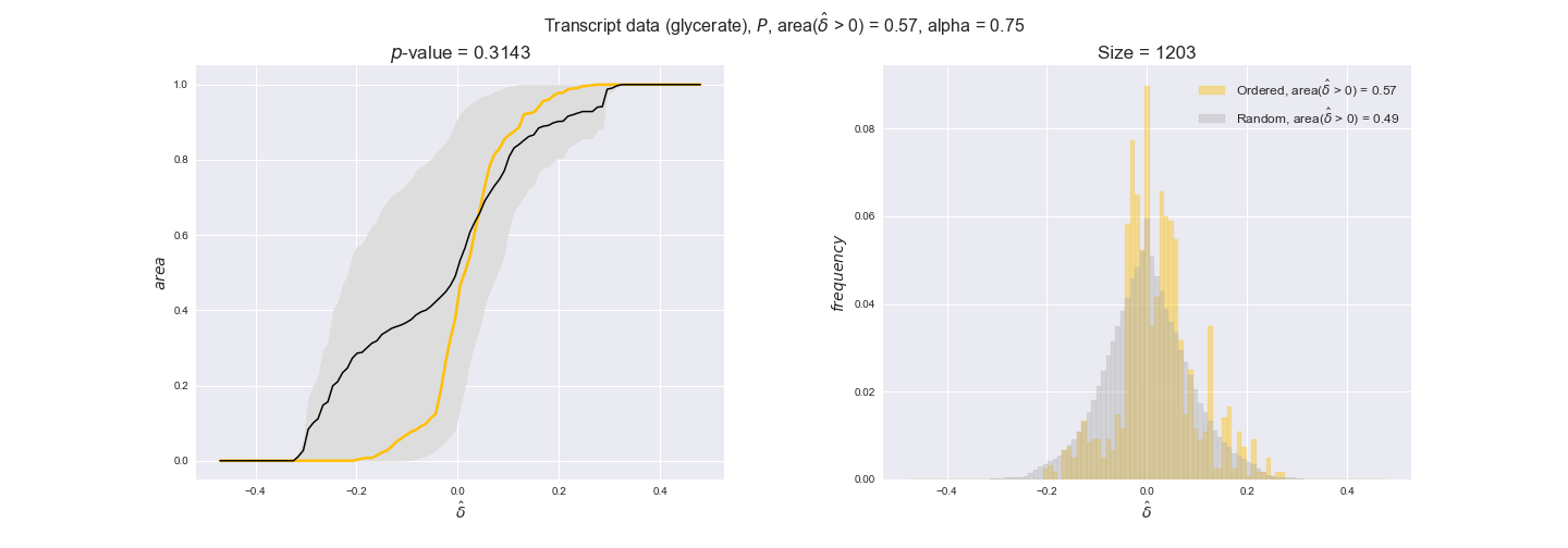


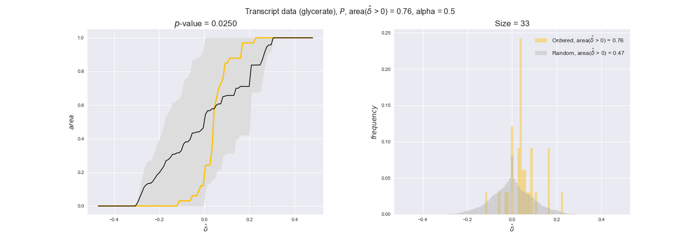
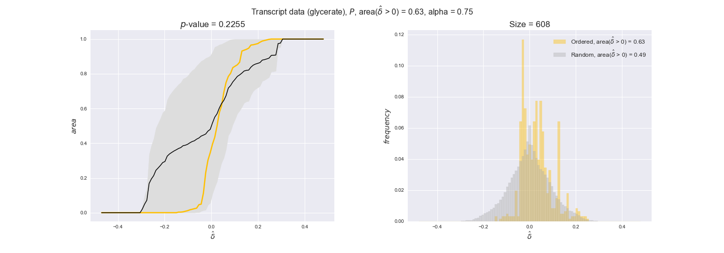
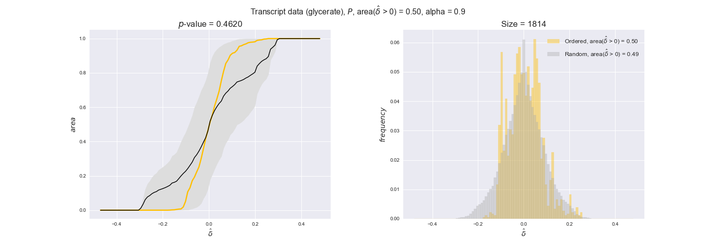
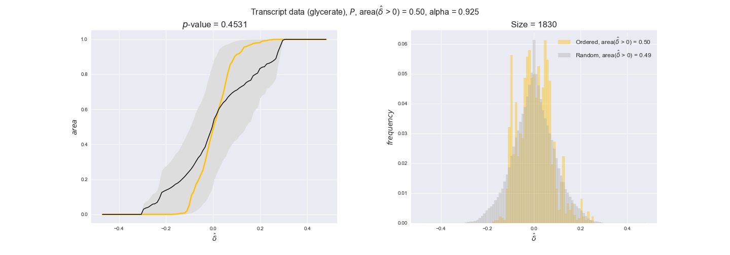

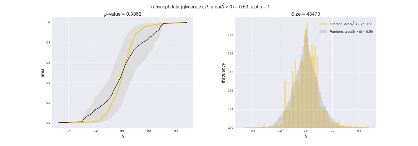
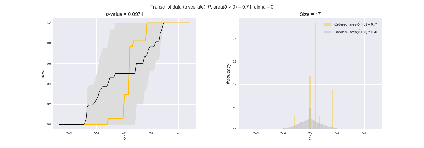
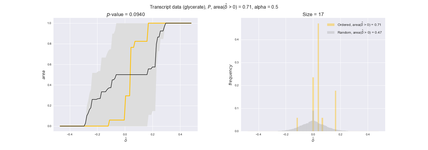
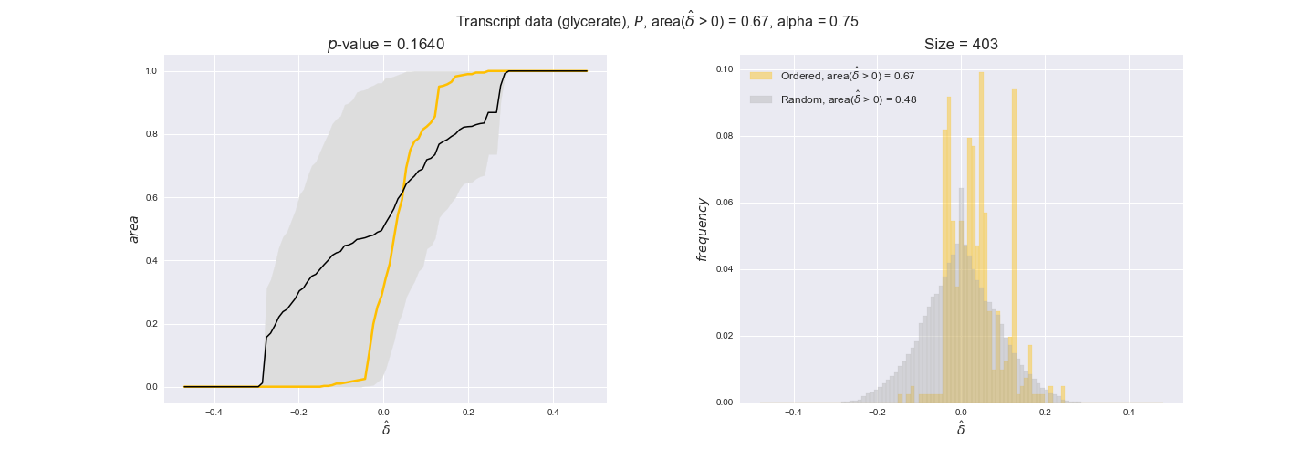

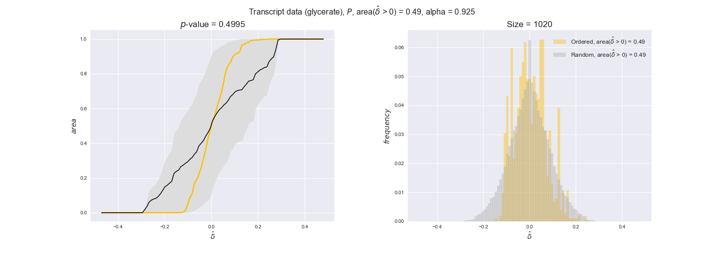
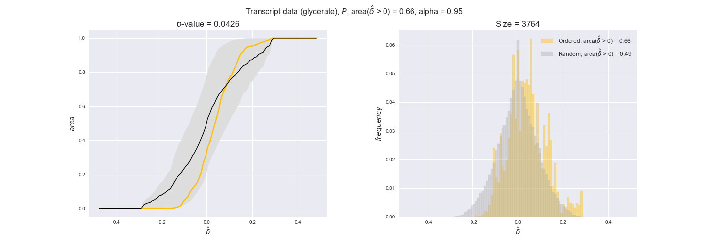
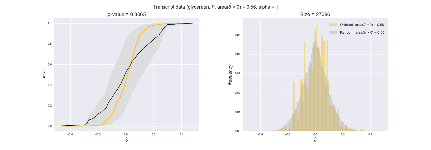
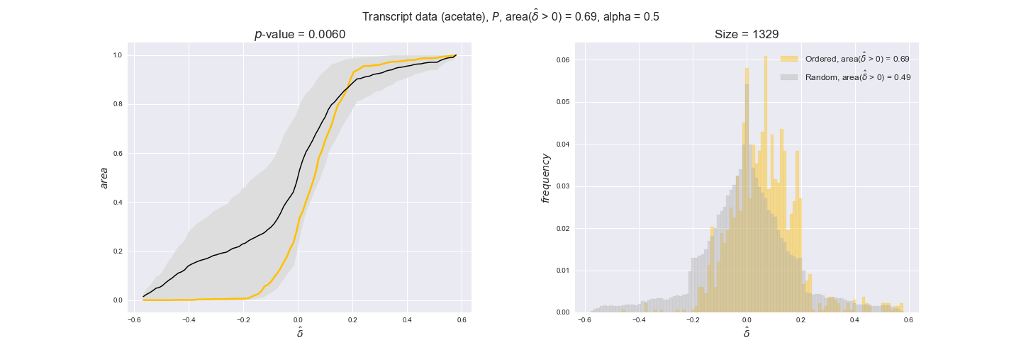

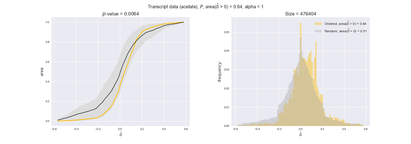
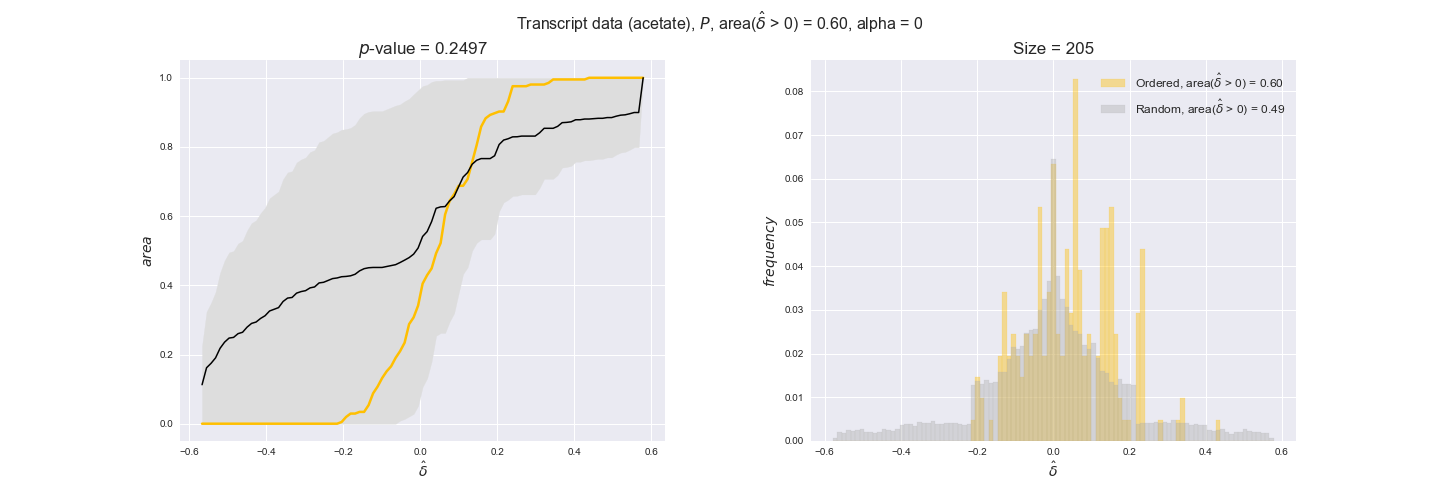
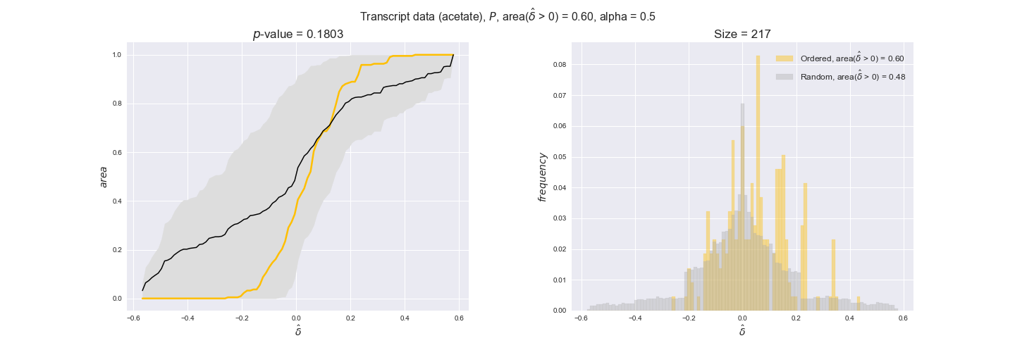
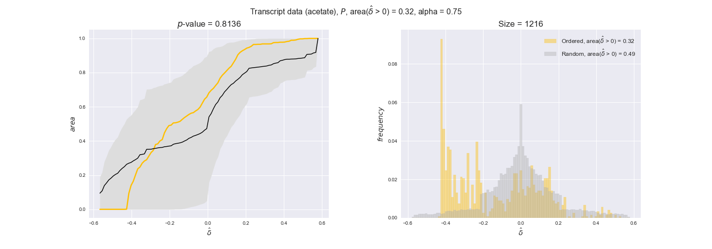
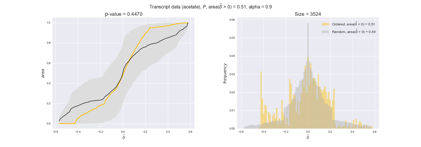

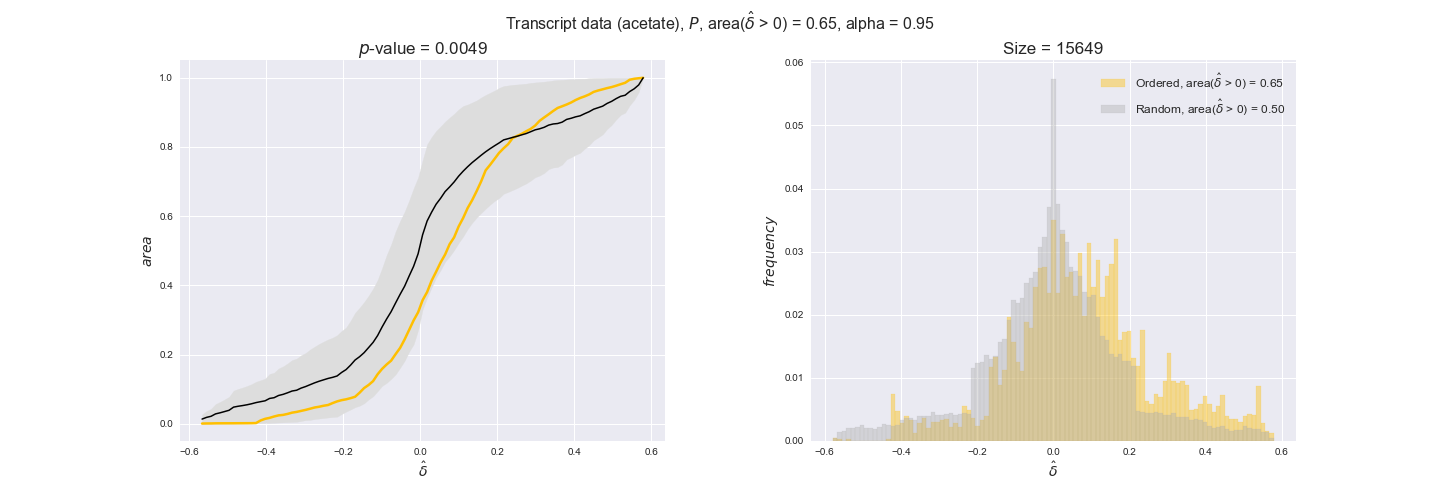
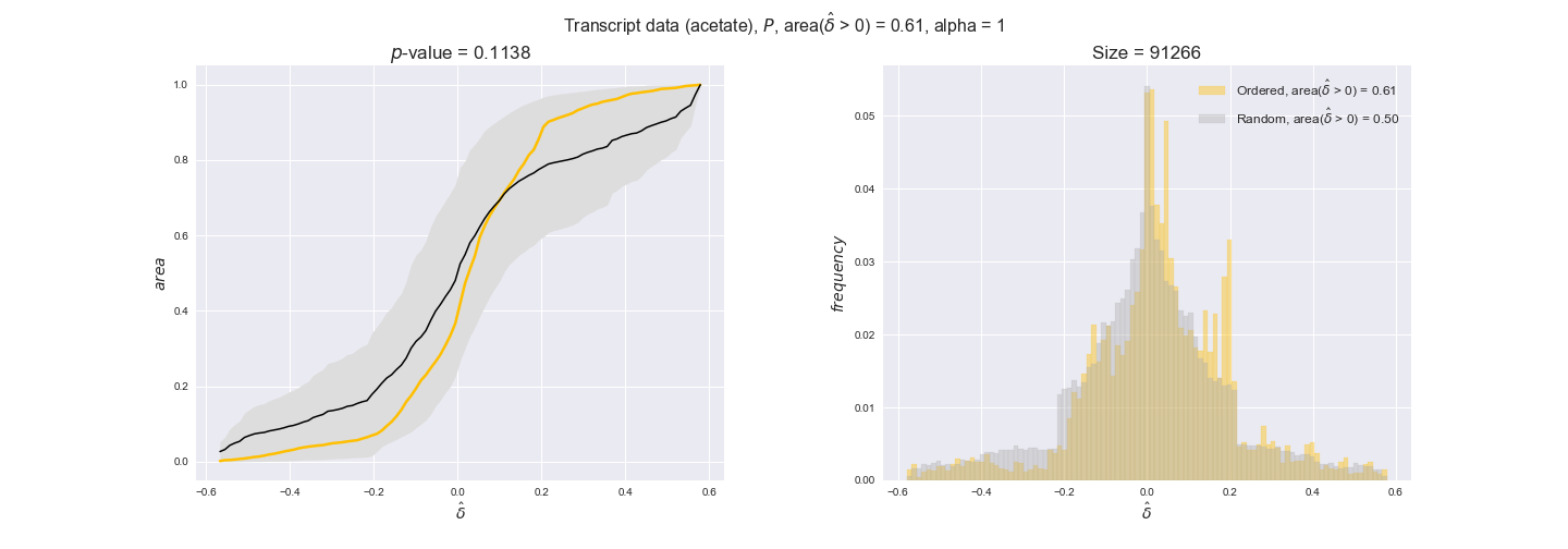
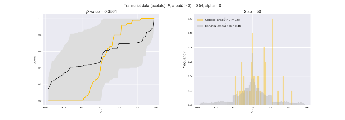
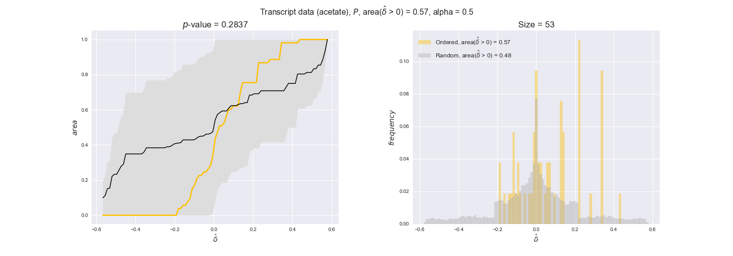
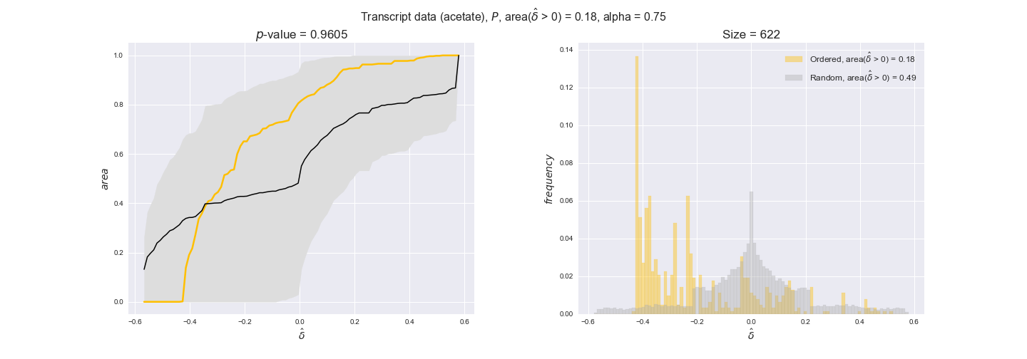

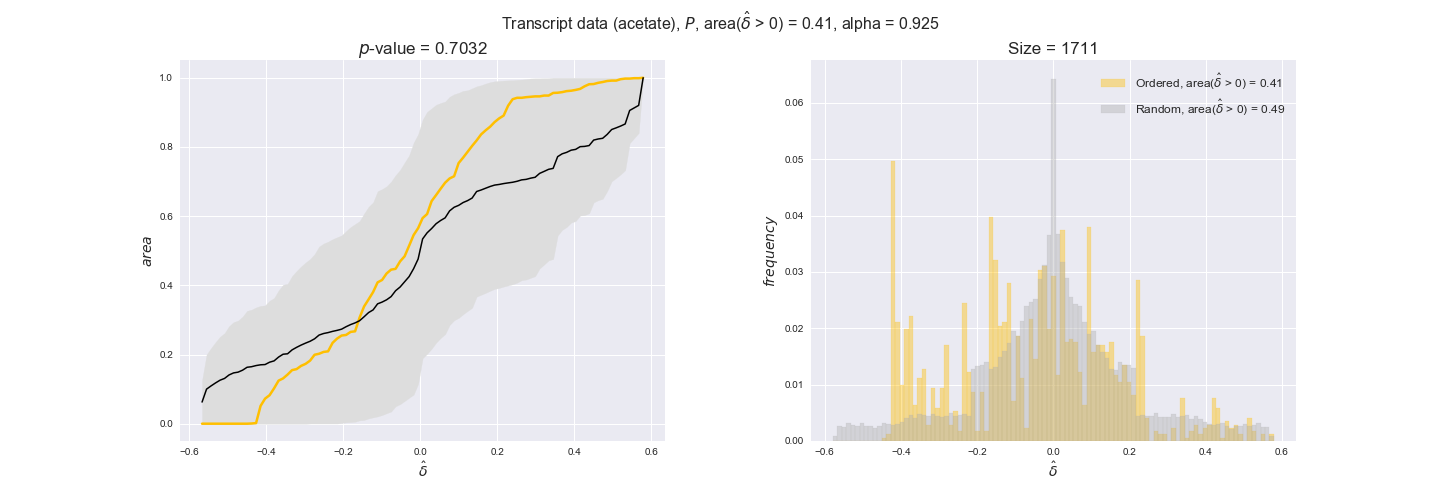
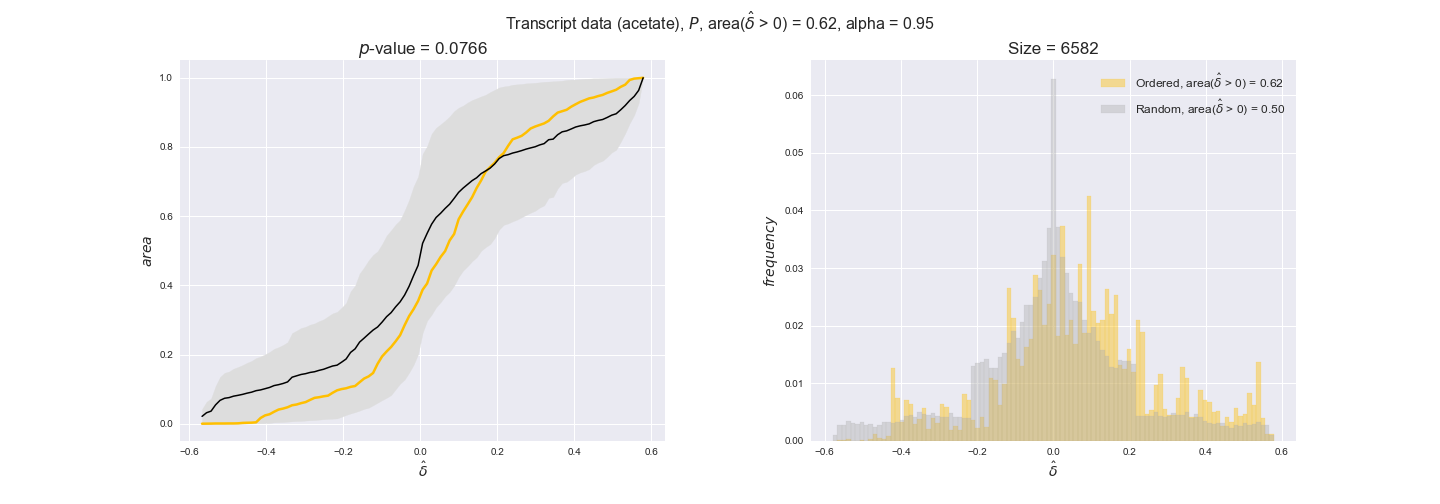

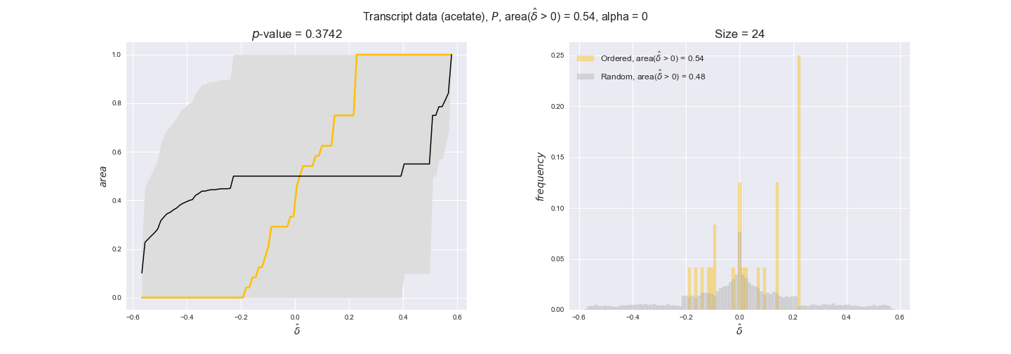
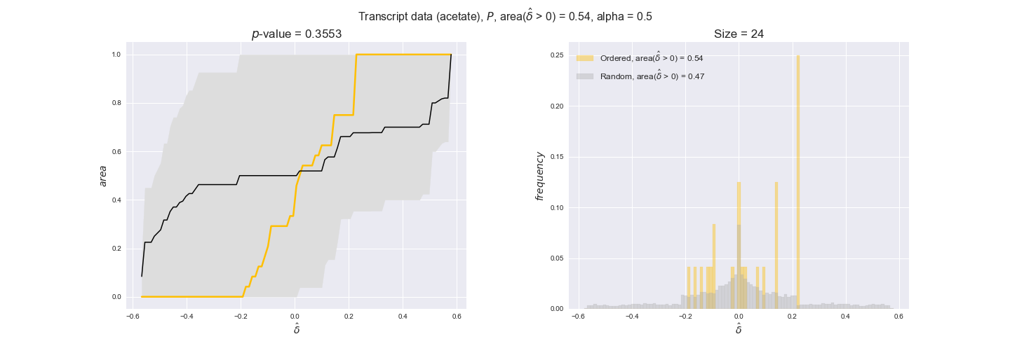
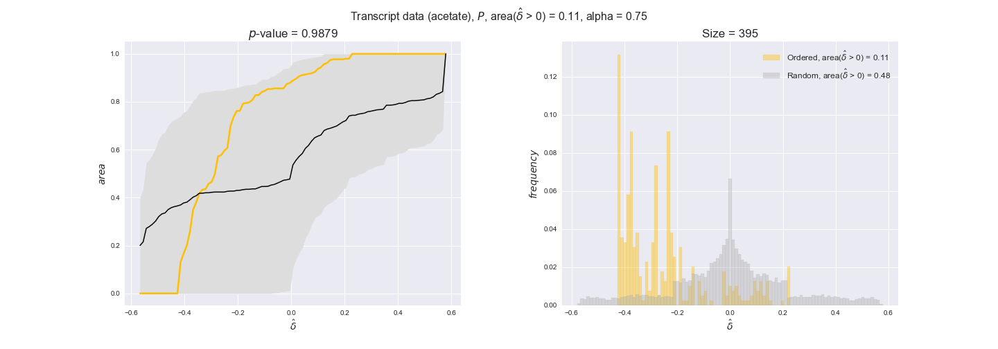
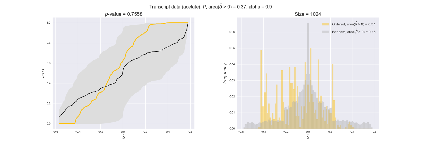
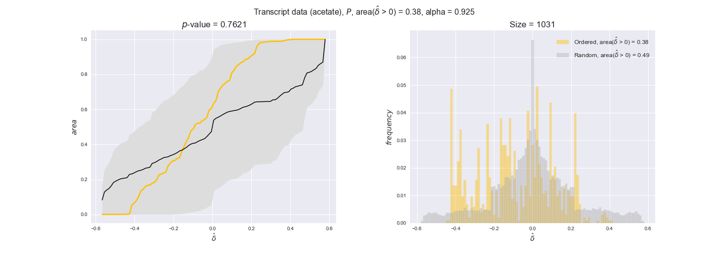
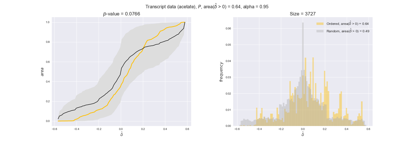
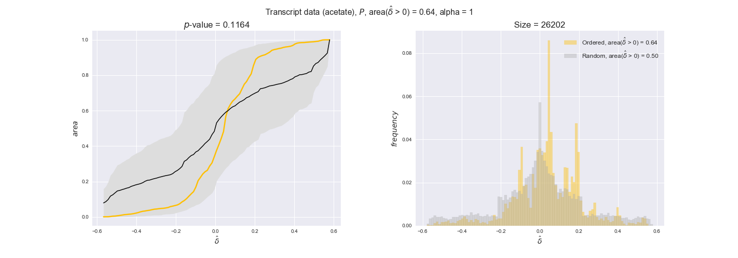
We begin analyzing growth on glucose when including all flux-ordered reaction pairs, i.e., the cost threshold is the $\mathrm{P}_0$ percentile of the cost distribution. We see that transcript levels follow the flux order relation in 63% of the cases and this result is significant with a fairly low experimental $p$-value = 0.0005, that's 5 times the minimum possible for this study. This result indicates that transcript levels do partially follow the flux-order relation, which is is line with the hypothesis that enzyme levels are regulated to match the flux order relation to avoid unnecessary (over)production of enzyme. What would happen if we selectively look at the sets of flux-ordered pairs with increasing enzyme costs? Upon changing the cost percentile, we can see that the fraction of average positive differences increases from 63% at $\mathrm{P}_0$ to 83% at $\mathrm{P}_{85}$. This result further supports our hypothesis, the expression of enzymes with greater costs is more strongly regulated to match the flux order relation as to minimize the total costs derived of producing unneeded enzyme units.
Results are not as clear, however, when we analyze the other two carbon sources. While data associated to flux-ordered pairs also tends to follow the flux order relation, the fraction of positive average differences stays unchanged across increasing cost thresholds, ranging from 62% to 66% in both carbon sources. It may be that enzyme costs, which are measured as moles of carbon source consumed per mol of protein synthesized, are more accurate in the case of glucose that in the case of acetate — there is not cost data for glycerate, we have employed glucose costs in this case. Let's continue our analysis with the protein data set which represent a better proxy of reaction fluxes.
protein_plots = pm.plotDataOrder(protein_plot_data, data_colors['protein'], interactive=True)
protein_plots
Percentile:
alpha (biomass):
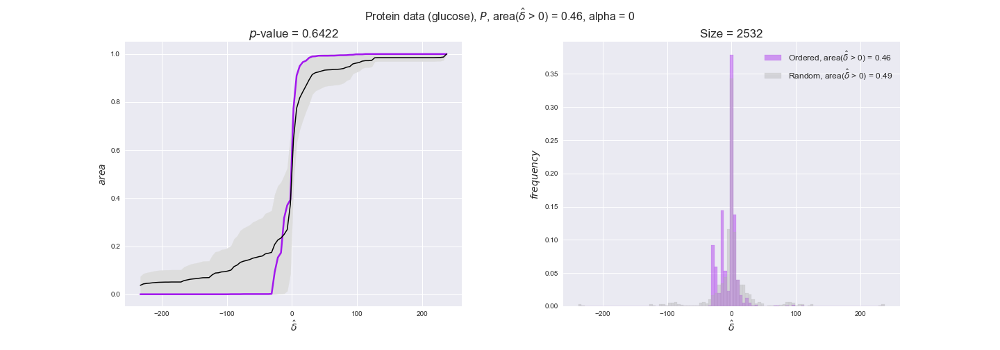
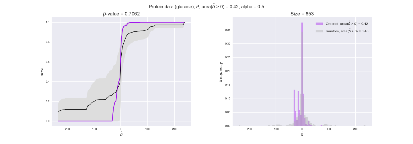
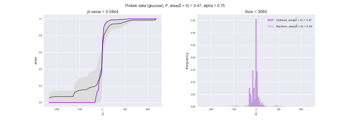
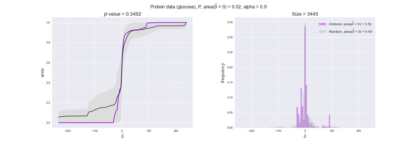

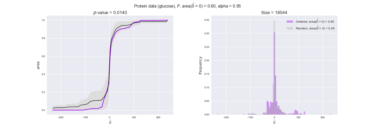
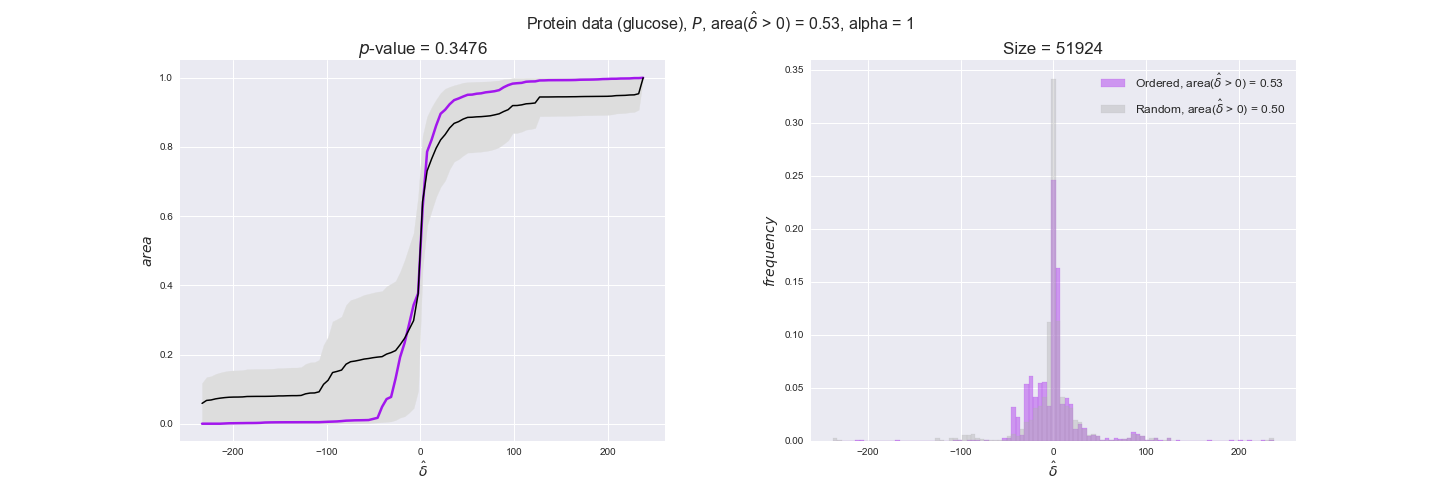
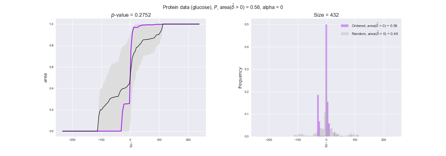


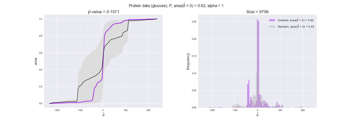
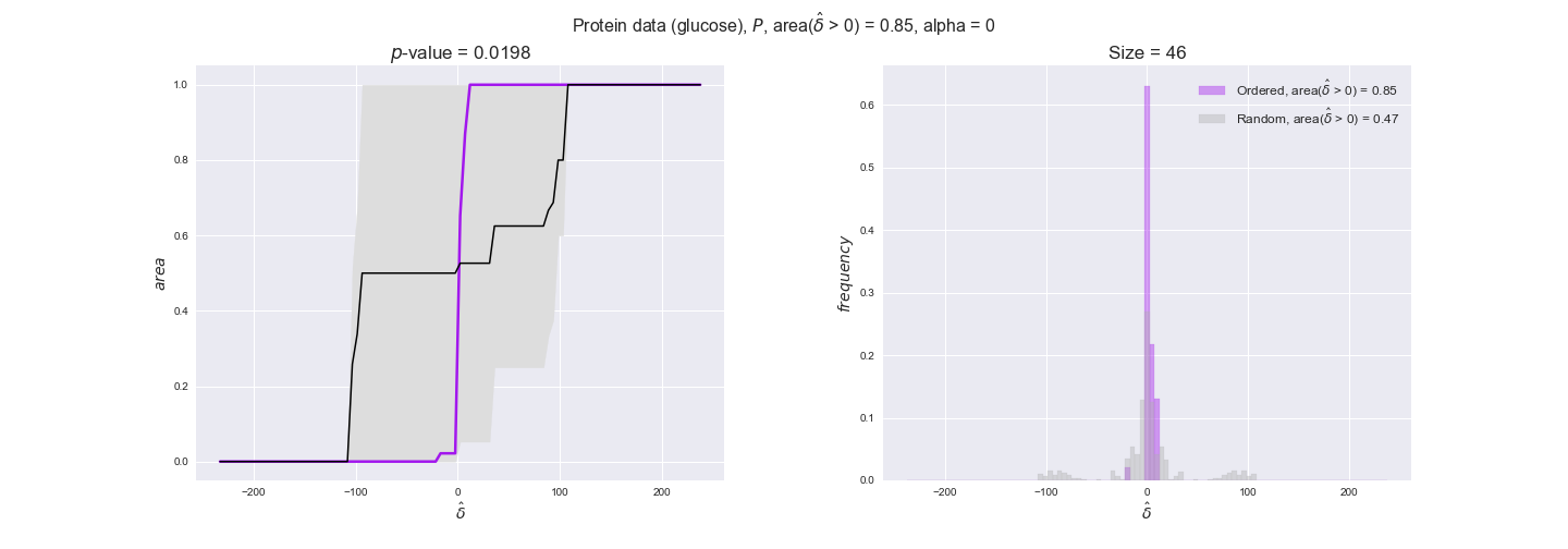


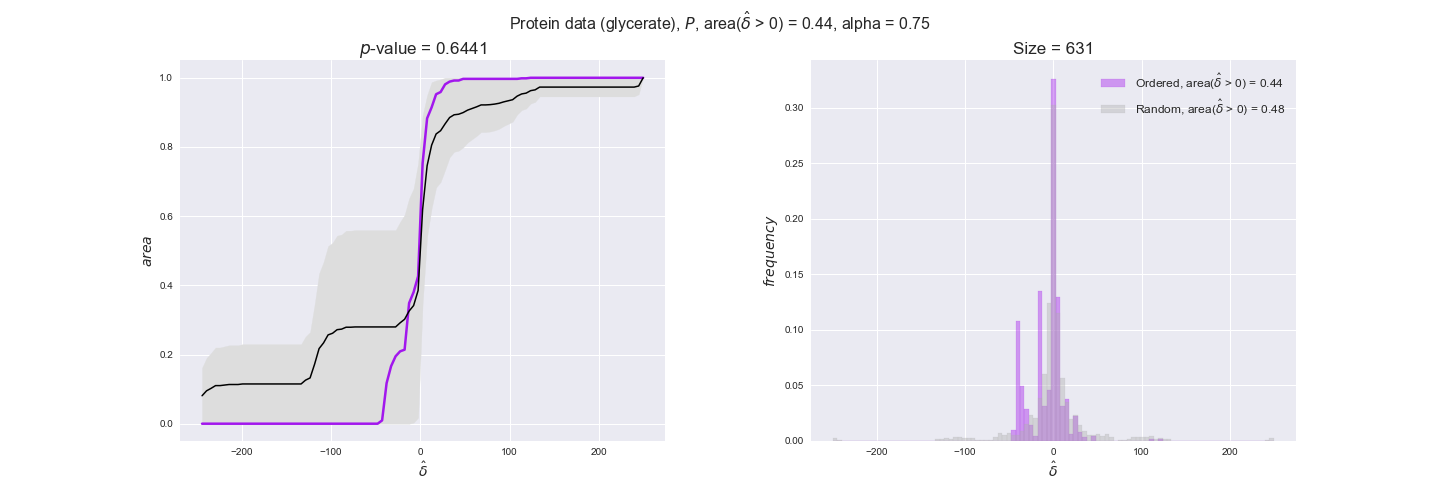
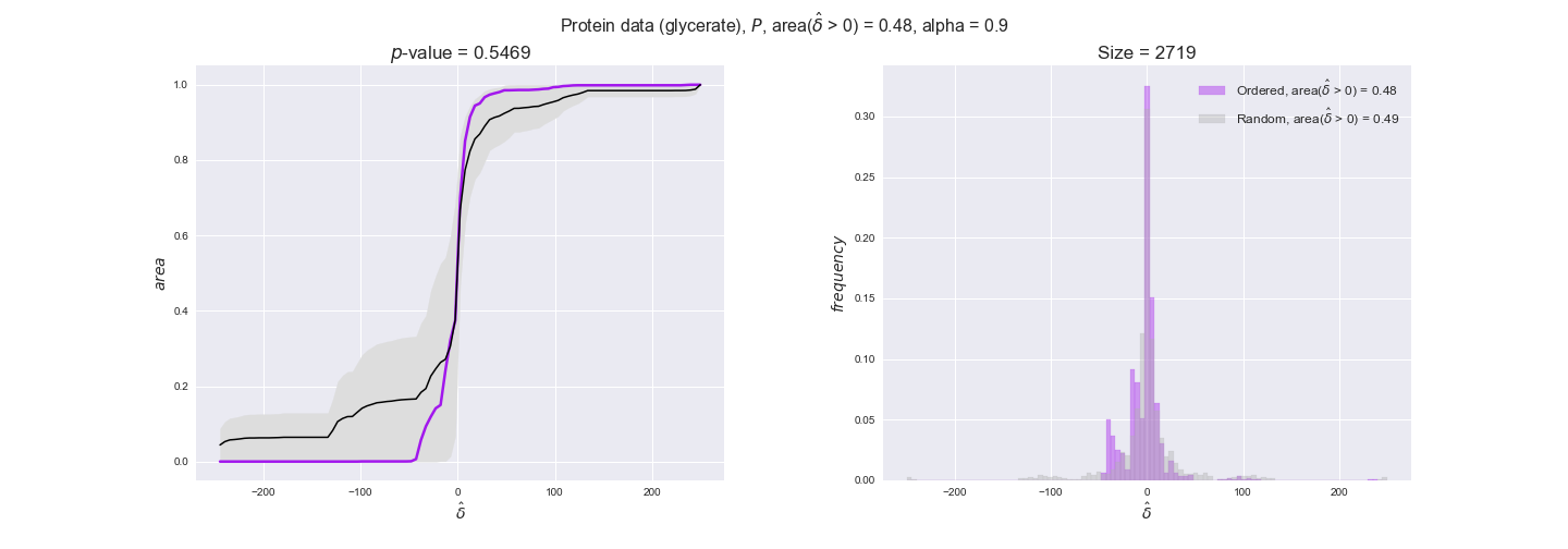
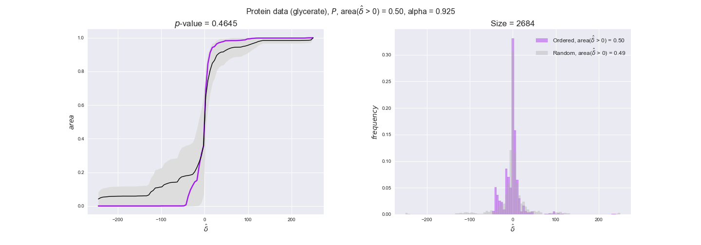
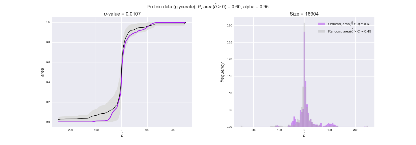
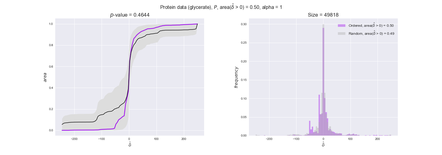

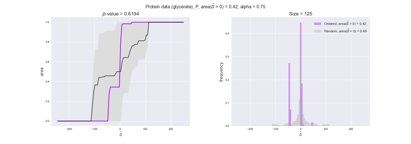
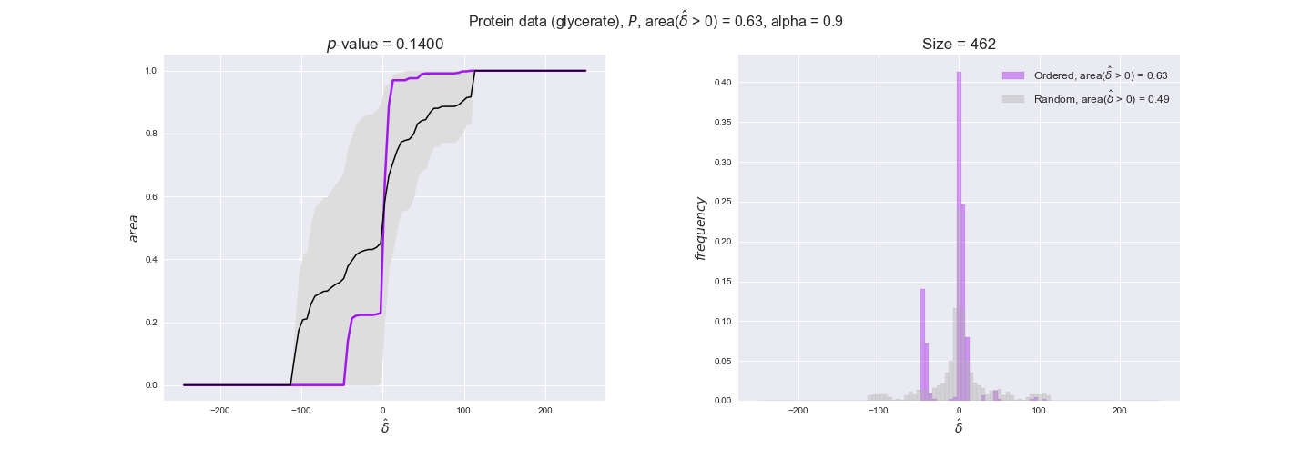
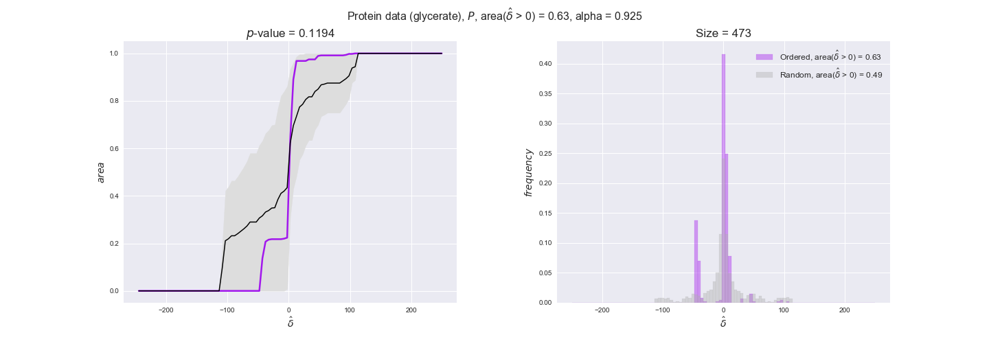
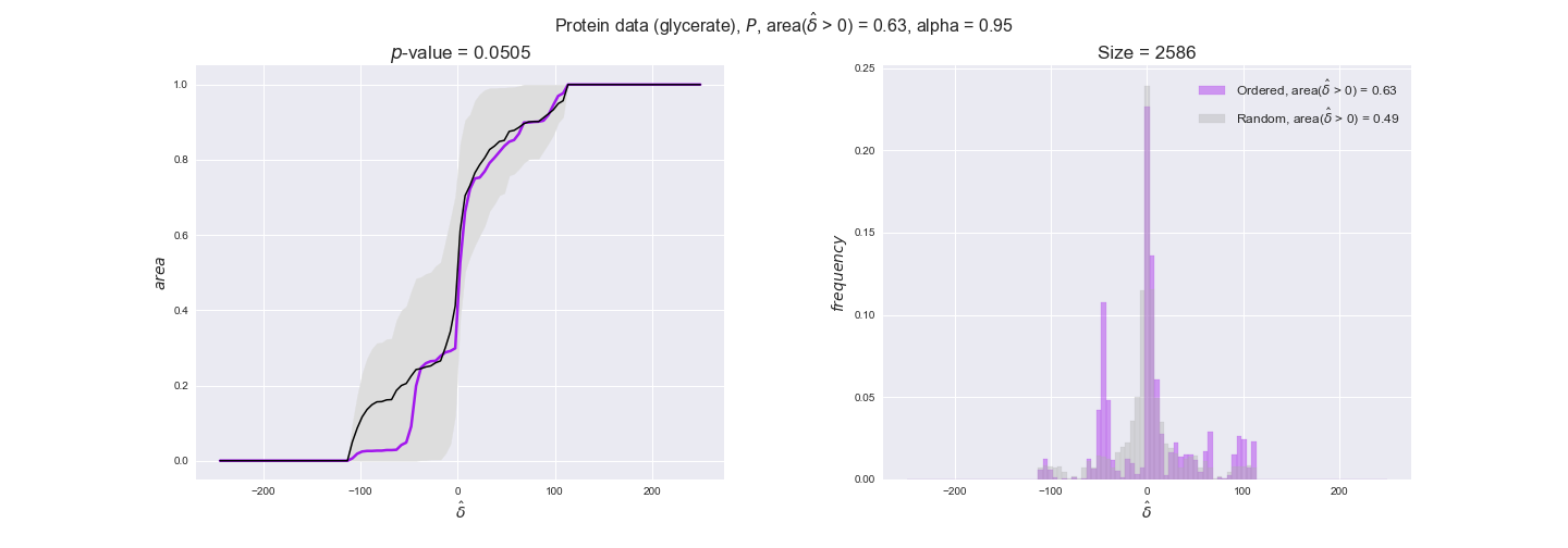
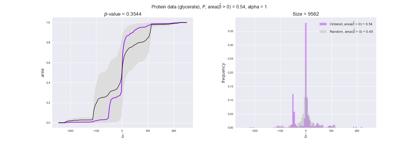


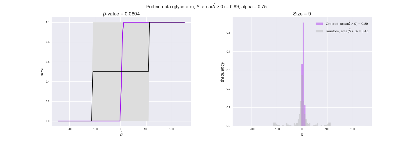
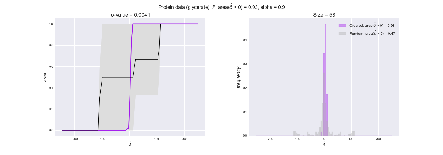
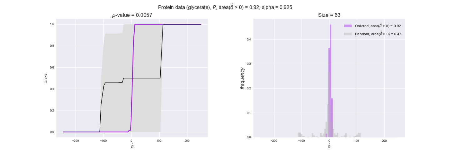
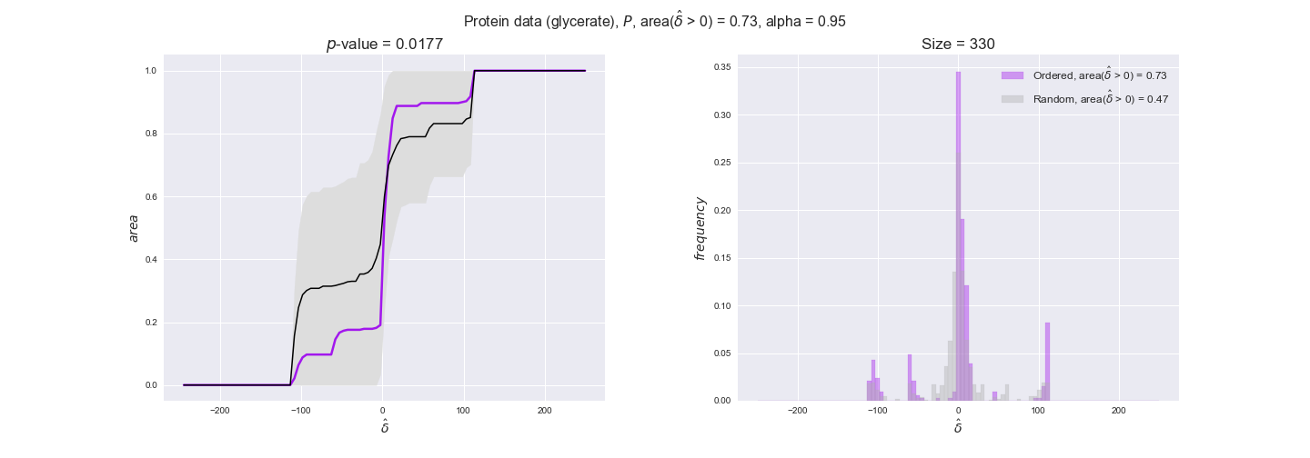
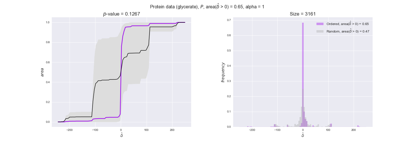


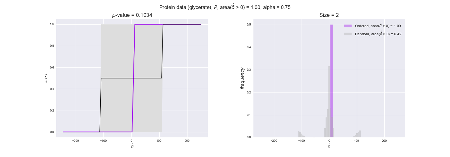

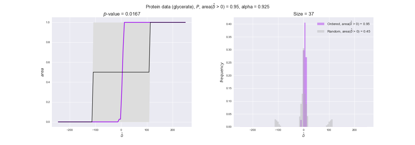
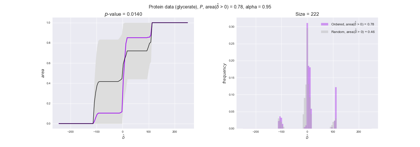
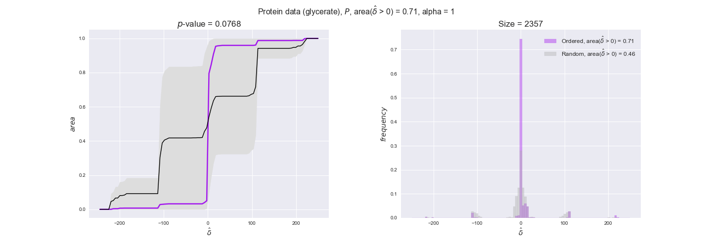


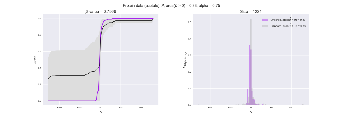
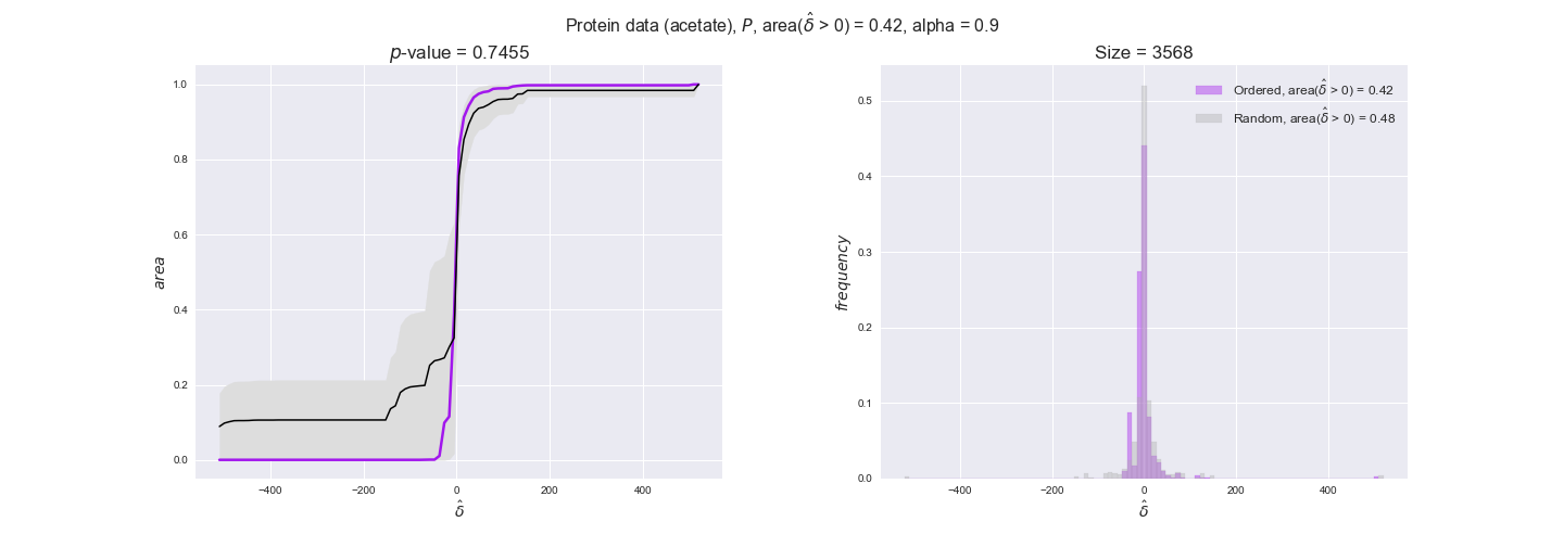
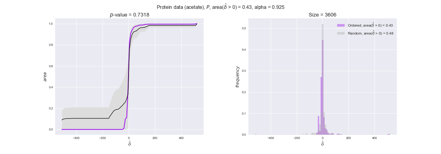
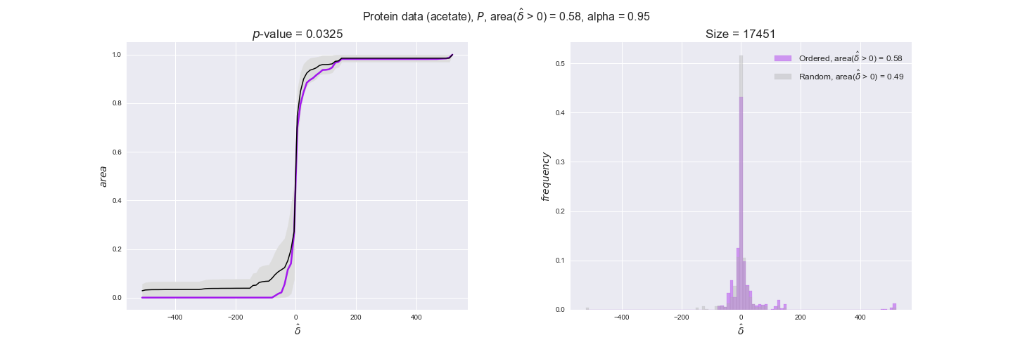
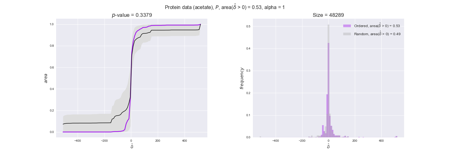


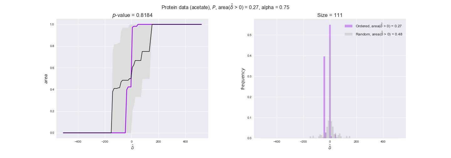
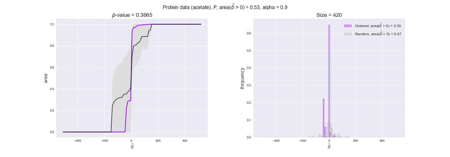

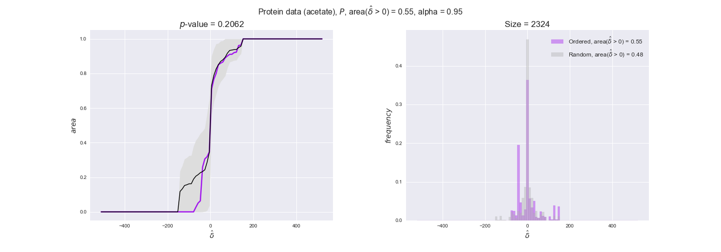
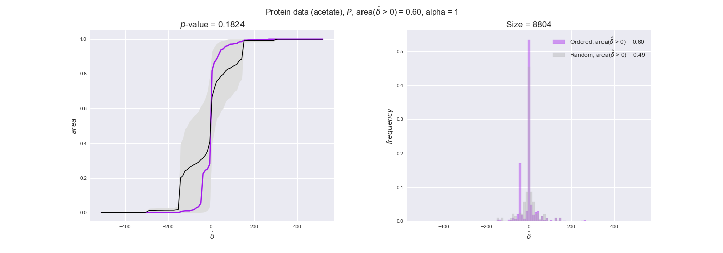


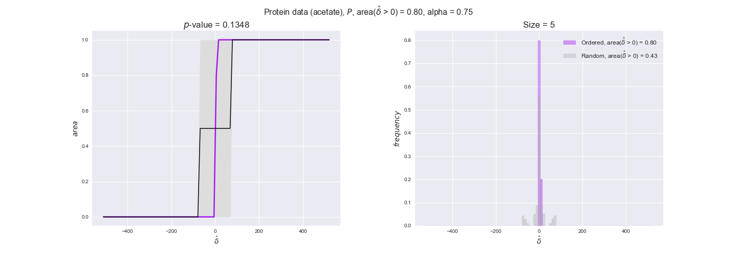
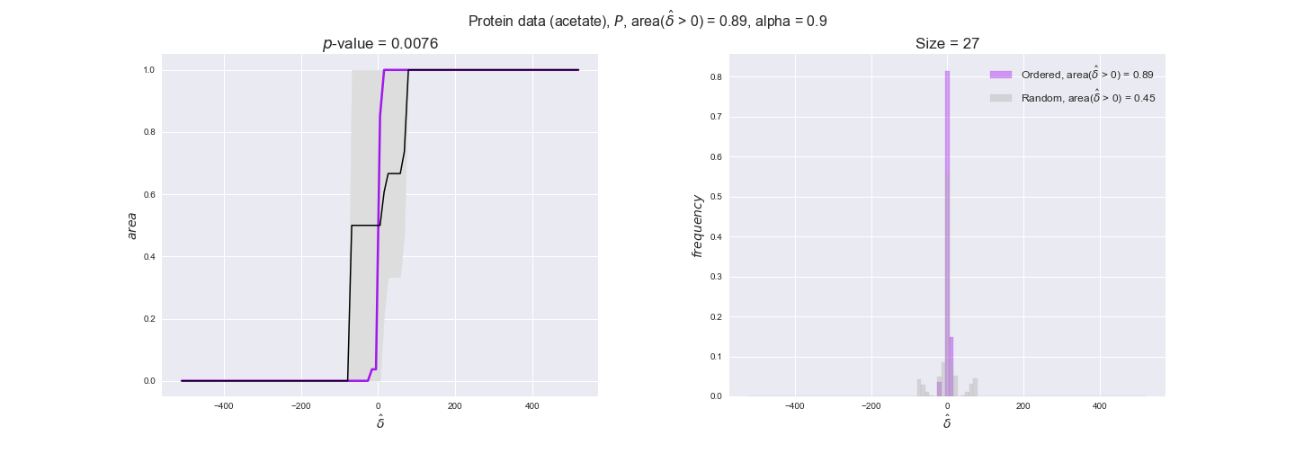
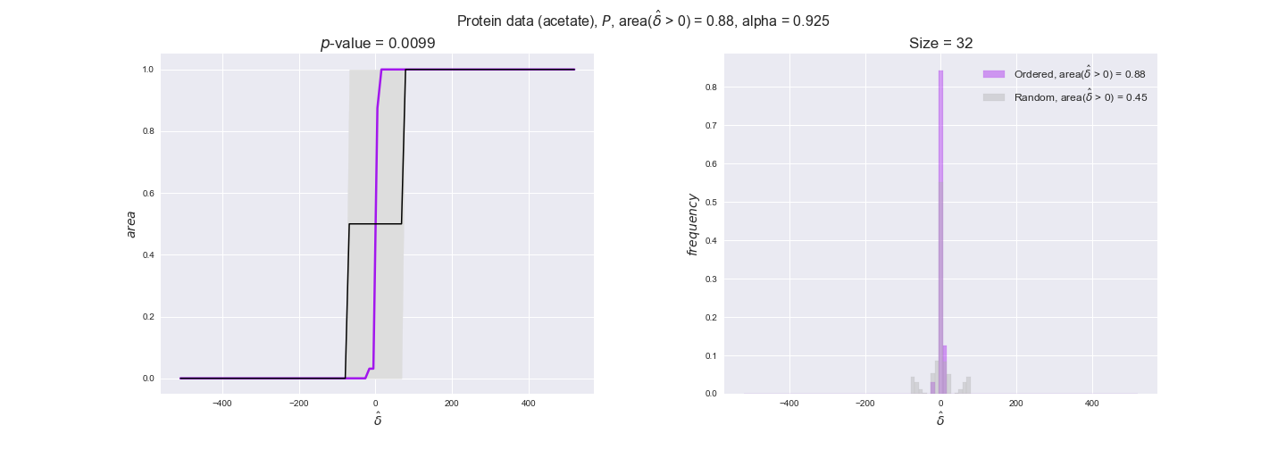
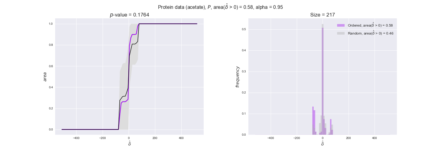


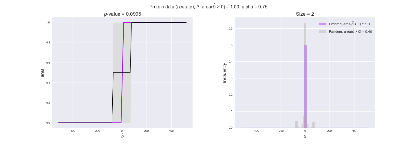
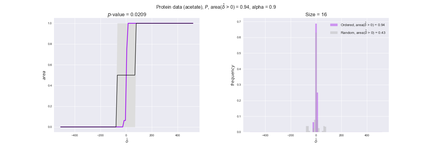

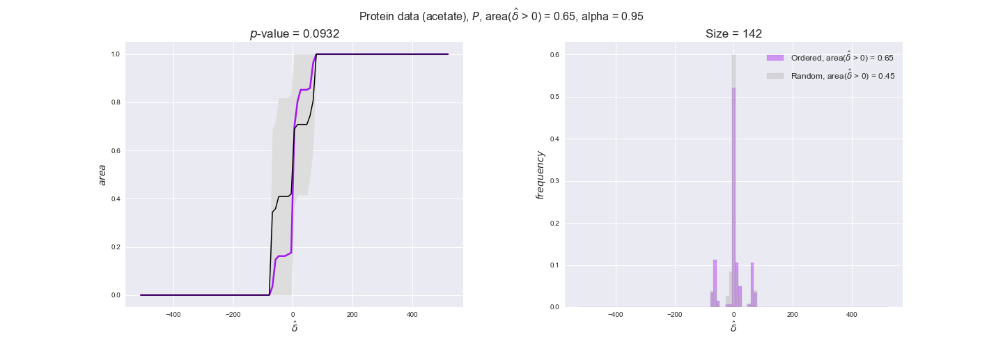
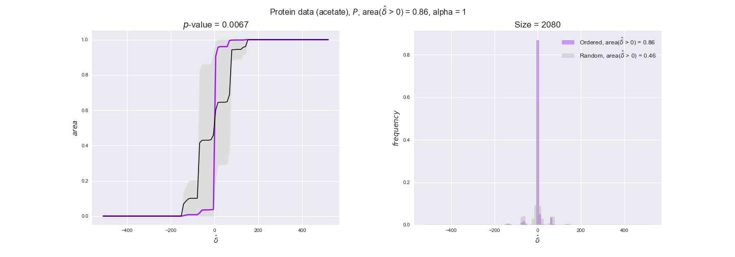
We observe that protein levels tend to follow the flux order relation in all three carbon sources, with fraction of positive average differences of 60% for glucose and glycerate and of 58% for acetate, and $p$-values ranging from 0.01 for glucose to 0.03 for acetate. Additionally, similar to transcript data, the fraction of positive differences grows with increasing enzyme production costs, although only in the case of glucose and glycerate as carbon sources. When employing acetate as carbon source, the fraction of positive differences is only significant at $\mathrm{P}_0$.
To conclude this section, we have seen that transcript and protein data follow the flux order relation to some extent. Additionally, in line with our hypothesis about minimizing enzyme production costs, data tend to better follow the flux order relation in the case of costly enzymes. However, the latter results only hold under glucose in the case of transcript data and glucose and glycerate in protein data.
3.3. Enzyme $k_{cat}$ values and the flux order relation
Finally, we consider a fundamental property of enzymes: the catalytic constant, $k_{cat}$. $k_{cat}$ values are ultimately result of physicochemical properties of the enzymes, and, hence, are not affected by enzyme regulation or by environmental effects such as the available carbon source. For this reason, we will test the same $k_{cat}$ data on all three sets of ordered pairs, one per carbon source. We should obtain similar results across carbon sources. We only have one data value per reaction, so here we compute the distribution of data differences $\delta$ instead of average differences as before.
kcat_plot = pm.plotDataOrder(kcat_plot_data, data_colors['kcat'], interactive=True, has_protein_costs=False)
kcat_plot
alpha (biomass):
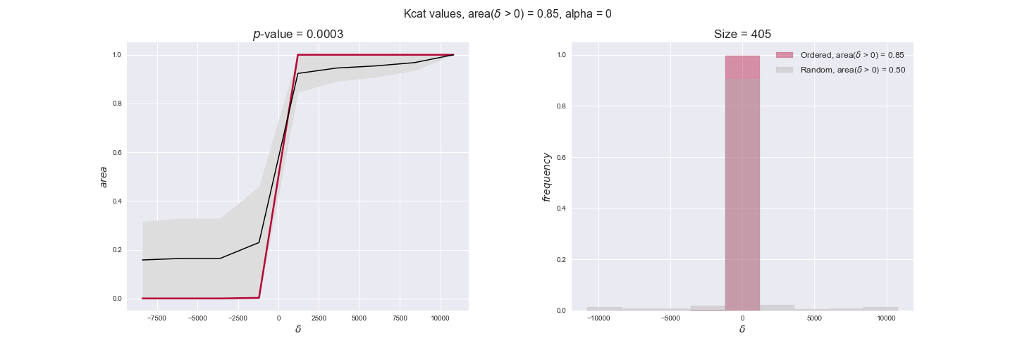
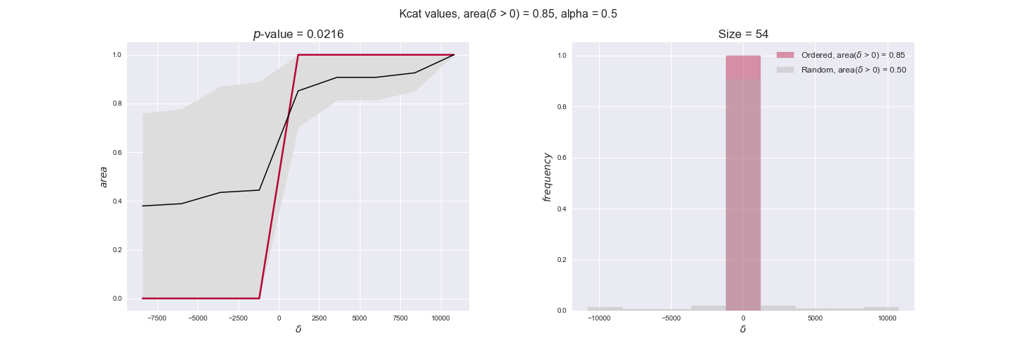


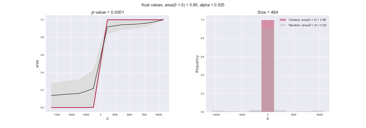
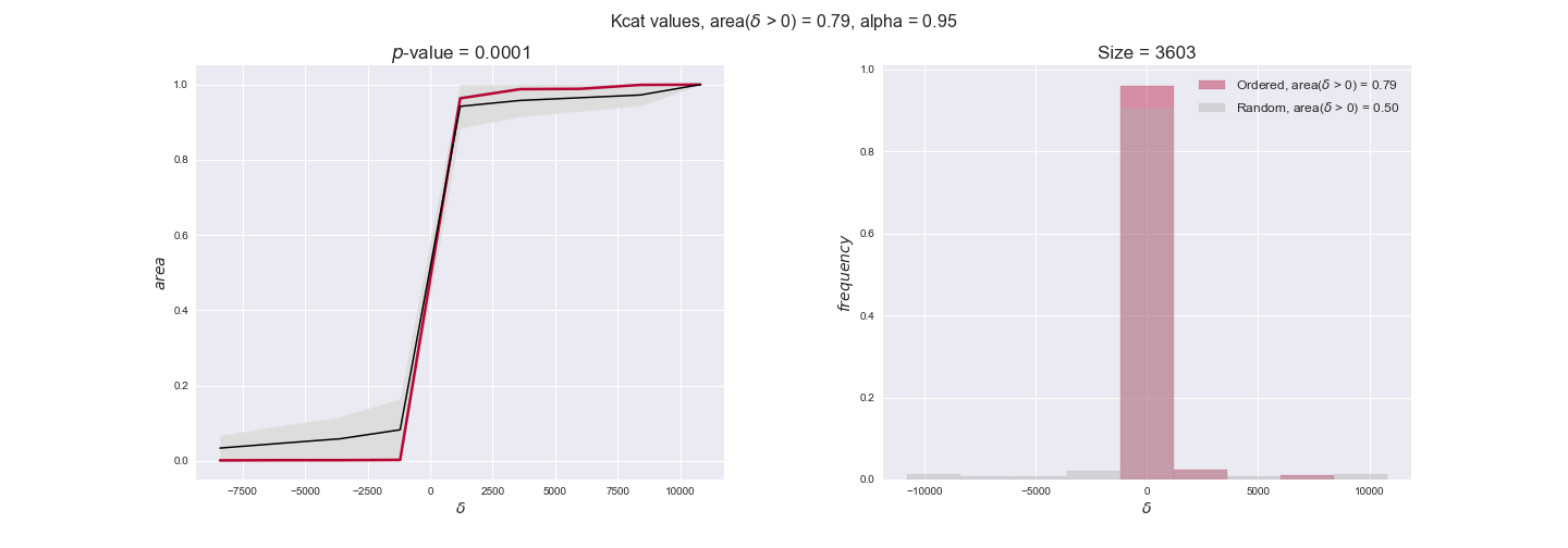
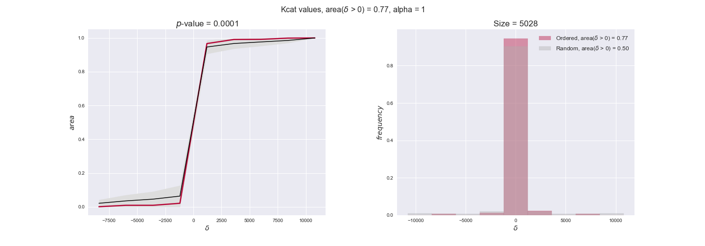


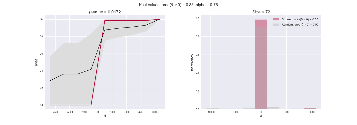


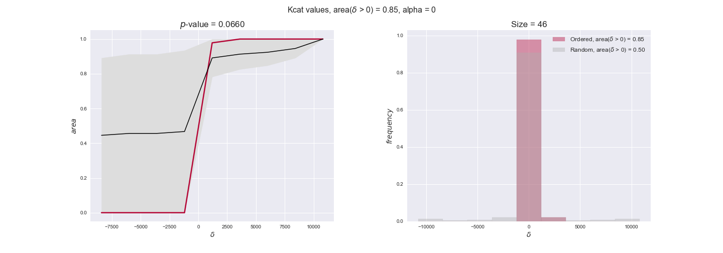
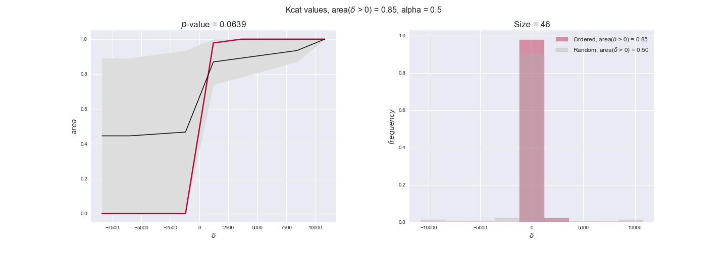
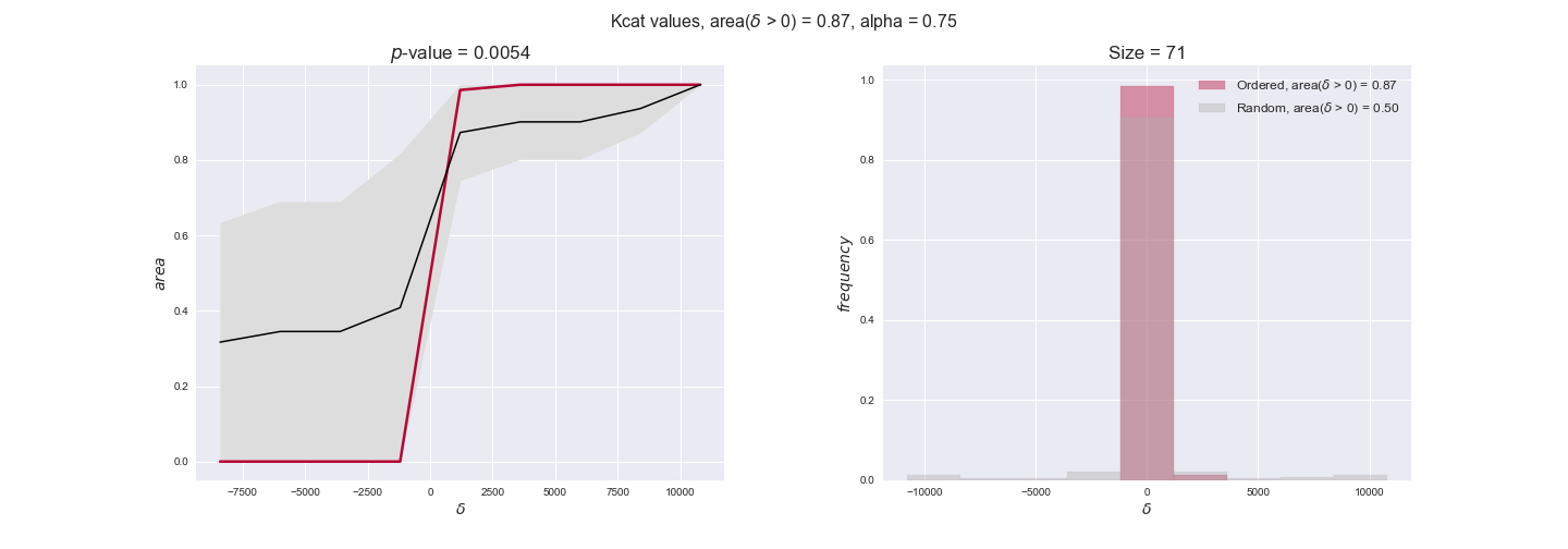
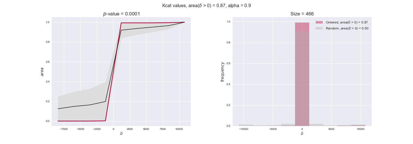
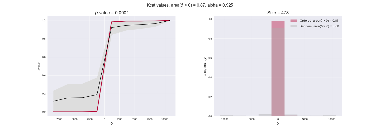
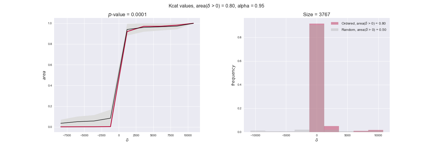
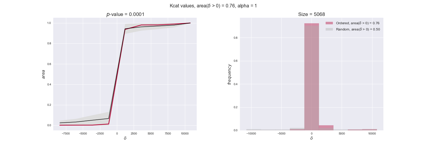
We see that $k_{cat}$ values produce positive differences in approximately 80% of the cases when we use models across carbon sources, thus suggesting that enzymes have optimized this property during evolution to match the flux order relation. Additionally, the $p$-value = $10^{-4}$ is the smallest possible, i.e. none of the samples in the permutation analysis produced an equal or more extreme observation, thus results are solid. There are two observations here. On the one hand, optimizing $k_{cat}$ values would further minimize metabolic costs since increasing reaction rate to match the order relation would be done by modifying the catalytic rate instead of the number of enzyme copies. On the other hand, there is experimental evidence indicating that many enzymes, particularly in central metabolism, operate under substrate saturation — in conditions in which reaction rate is independent of substrate concentrations. In this latter case, $k_{cat}$ values correlate even better with reaction fluxes since reaction fluxes no longer depend on metabolite concentrations.
3.4. Gene regulatory interactions and the flux order relation
Reactions situated in higher positions in the hierarchical graph depicting the flux order relation control the flux upper bound of larger sets of reactions than those situated in lower positions. Hence, by regulating the activity through reactions in upper levels, a cellular system could more efficiently control the flux through the metabolic network. We will next investigate whether coding genes of enzymes catalyzing reactions in upper layers tend to be more transcriptionally regulated than those situated in lower levels. To this end, we will partition the 19 levels of the flux order DAG corresponding to glucose into three groups which roughly contain the same number of reactions: the first, middle and last group. As discussed in the introduction to this section, we consider here the total number of regulatory interactions per gene, i.e., both activating and inhibtory. Let's (box)plot the distributions of total number of regulatory interactions per group.
# Evaluate regulatory interactions in the flux order DAG
GraphDataEvaluator = DataOrderEvaluator(iJO1366_Orders_DataFrame, Model=iJO1366['glucose'], data=geneRegulationData)
evalFluxOrderRegulations = GraphDataEvaluator.evaluateGeneDataPerGraphLevel(
        Graph_Levels['glucose'], statistic='mean', sampleSize=10,
        plotTitle='Flux orders', group_levels=True)

for comparison in evalFluxOrderRegulations['pvalues']:
    print('Level {} > {}, with p-value = {}'.format(comparison[0][0], comparison[0][1], comparison[1]))

It seems like the genes of reactions in the first and middle groups tend to be more regulated than those in the last group while the first and middle groups look alike. After applying a one-sided Mann-Whitney test, we obtain significant $p$-values only in the first-last and middle-last comparisons.
A similar analysis was conducted in , where authors reconstructed the directional flux coupling DAG corresponding to E. coli's metabolic network. Authors found a positive association between the DAG level and the gene regulation state (regulated vs no regulated). Hence, we conducted a similar analysis and reconstructed the directional flux coupling DAG of of E. coli, employing this time the same data set as before: total number of regulatory interactions per gene. We will next reconstruct the flux-coupling DAG.
# Reconstruct the flux-coupling DAG
iJO1366_B = hm.getDirectionalCouplingAdjacencyMatrix(iJO1366_fctable)

iJO1366_Coupling = FluxOrder(iJO1366['all'], AdjacencyMatrix=iJO1366_B, fctable=iJO1366_fctable)
Coupling_Graph = iJO1366_Coupling.getGraph()
Coupling_Graph_Levels = Coupling_Graph.getGraphLevels()
Coupling_Levels = {'all': Coupling_Graph_Levels}
df = pm.plotNumberOfReactionsPerGraphLevel(Coupling_Levels)
print('There are a total of {} reactions in the flux coupling DAG'.format(df.sum()[0]))

Our flux-coupling DAG contains a total of 1590 reactions distributed across 8 graph levels. Similar to the flux order DAG, the first two levels contain the majority of reactions in the DAG. Let's now evaluate whether, here too, the number of gene regulatory interactions is higher in the first levels in comparison to the last levels.
# Evaluate regulatory interactions in the directional coupling DAG
iJO1366_CouplingDataFrame = hm.getFluxOrderDataFrame(iJO1366_B, iJO1366['all'])
GraphDataEvaluator = DataOrderEvaluator(iJO1366_CouplingDataFrame, Model=iJO1366['all'], data=geneRegulationData)
evalCouplingRegulations = GraphDataEvaluator.evaluateGeneDataPerGraphLevel(
        Coupling_Graph_Levels, statistic='mean', sampleSize=10,
        plotTitle='Flux coupling', group_levels=True)

for comparison in evalCouplingRegulations['pvalues']:
    print('Level {} > {}, with p-value = {}'.format(comparison[0][0], comparison[0][1], comparison[1]))

We obtain a result that is qualitatively identical to the one obtained with the flux-order DAG. Namely, genes of reactions in the first and middle groups of levels show significantly larger numbers of total gene regulatory interactions. These results are also aligned with the ones obtained in .
To conclude this section, we have seen that diverse types of experimental data tend to respect the flux order relation. ${}^{13}\mathrm{C}$-derived flux levels are the only data type that can directly reflect the flux order relation and, indeed, we saw that they match the flux order relation in all cases. However, we have also seen that other, indirect measurements of flux levels tend to follow the flux order relation. This is particularly marked in the case of enzyme specific activities, $k_{cat}$ values and transcript and protein data when enzyme production costs are high. These observations support the hypothesis that E. coli has evolved to sustain enzyme levels and activities that match the flux order relation to avoid the overproduction of unnecessary enzyme units, hence minimizing costs. Finally, we saw that genes of reactions situated in the first levels of the flux order DAG tend to be more regulated, at least to some extent, than those of reactions in the last levels. This observation aligns with the fact that reactions in higher positions in the DAG have a greater capacity to control metabolic flux, since they constrain the flux of a greater number of reactions.
4. On reaction essentiality
Identifying essential reactions — reactions that must carry non-zero flux to enable cellular growth — is crucial in both biotechnological and biomedical settings. For instance, in the first case, essential reactions and their genes form a set that cannot be removed during metabolic pathway optimization approaches. In the second case, essential reactions and their enzymes provide potential targets to halt the growth of pathogens .
All reactions that are flux-ordered with the biomass (pseudo)reaction are also essential, due to the flux upper bound imposed on biomass production. However, it is unclear whether all essential reactions are also flux-ordered with the biomass reaction. We will next investigate to what extent essential reactions are also flux-ordered with the biomass reaction. To this end, we will evaluate the intersection between the set of all reactions that are essential for growth on glucose — identified with cobrapy's native find_essential_reactions — and then of flux-ordered and essential reactions, i.e., all ancestors of the biomass reaction in the flux order DAG corresponding to glucose. Let's first compute the set of essential reactions and continue extracting the subDAG formed by all ancestors of the biomass reaction in the flux order DAG.
# Extract subDAG of biomass ancestors
biomass_rxn_id = 'BIOMASS_Ec_iJO1366_WT_53p95M'
G = iJO1366_Orders_DAG['glucose'].G
Ordered_essential_reactions = nx.ancestors(G, biomass_rxn_id)
Ordered_essential_reactions.remove('ATPM')
Ordered_essential_reactions.add(biomass_rxn_id)
Essential_G = G.subgraph(Ordered_essential_reactions)
# nx.write_gml(Essential_G, path='Essential_G.gml')

# Compute essential reactions using cobrapy
FBA_essential_reactions = find_essential_reactions(iJO1366['glucose'].GEM)
FBA_essential_reaction_ids= set([rxn.id for rxn in FBA_essential_reactions])
Essential_reactions_intersect = FBA_essential_reaction_ids.intersection(Ordered_essential_reactions)

n_essential = len(FBA_essential_reactions)
n_essen_ord = len(Essential_reactions_intersect) - 1
print(('There are a total of {} essential reacitons '
       'out of which {} are also flux-ordered with '
       'the biomass reaction').format(n_essential, n_essen_ord))
We see that all 27 reactions which are flux-ordered with the biomass reaction are also essential — Note that we removed the ATP maintenance (ATPM) reaction from the set since we imposed a lower flux bound greater than the biomass maximum, hence rendering it artificially flux-ordered, see accompanying paper for details. The code above generates a GML (Graph Markup Language) file which we can import into Cytoscape to generate a graph with a nice, hierarchical layout:
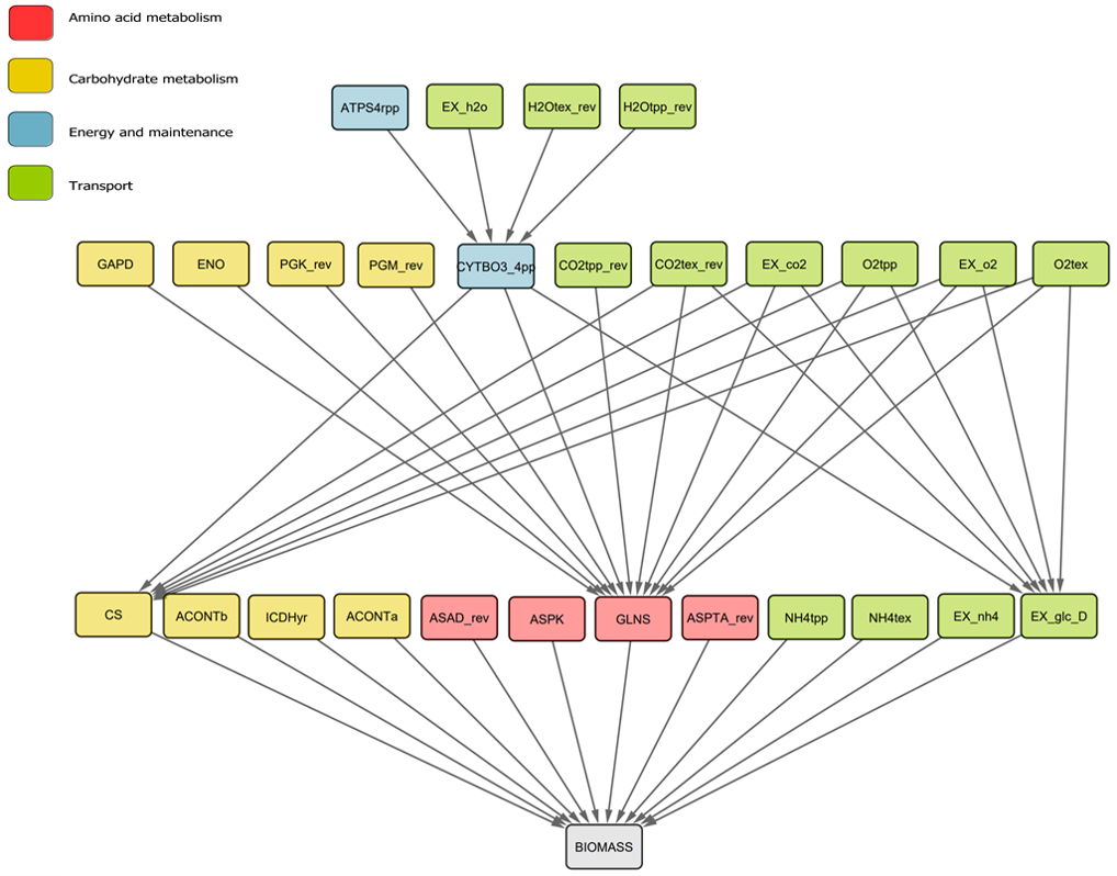
These are all the ancestors of the biomass reaction in the flux order DAG. Note that reactions are colored based on their metabolic macrosystems. It is not surprising to see that the four represented macrosystems: Transport, Carbohydrate metabolism, Aminoacid metabolism and Energy and maintenance are all critical to sustain growth.
We saw that the majority of essential reactions are not flux-ordered, however, this result is counterintuitive, provided that the flux order relation imposes an upper flux bound on the biomas reaction. We can understand the previous result by visualizing the flux space of two different reactions with the biomass reaction: one reactions which is only essential and another that is essential and flux-ordered with the biomass reaction. Let's start with reaction Geranyltranstransferase (GRTT), a reaction that is only essential.
# Plot only essential solution space
rxn_i_id = 'GRTT' #list(FBA_essential_reactions)[4]  # essential but not ordered
pm.plotSolutionSpace(iJO1366['glucose'].GEM, rxn_i_id, biomass_rxn_id, v_i_max=3,
                  n_points=100, plot_diagonal=True, r_j_nickname='Biomass',
                  plot_title='Only essential')

In this case, we see that the pair of reactions take flux values which are both above and below the line of equal fluxes $v_i = v_j$ (green dotted line) and the flux through biomass abruptly becomes zero when $v_{GRTT} = 0$. Hence, reaction GRTT is essential but cannot be flux-ordered. Let's now pick a reaction from the set of essential and flux-ordered reactions:
# Plot ordered and essential solution space
rxn_i_id = 'GLNS'  # ordered and essential
pm.plotSolutionSpace(iJO1366['glucose'].GEM, rxn_i_id, biomass_rxn_id, v_i_max=8,
                  n_points=100, plot_diagonal=True, r_j_nickname='Biomass',
                  plot_title='Essential and ordered')

We have picked reaction Glutamine synthetase (GLNS), in this case, we see that the flux space of the two reactions is always below the green dotted line, hence $v_{GLNS} \geq v_{Biomass}$ holds in any steady-state and GLNS is both essential and flux-ordered with the biomass reaction.
5. Conclusions
As a final conclusion, we have shown that the metabolic network of E. coli displays a new property when operating at steady state: the flux order relation, by which the flux values of some reaction pairs are always ordered, i.e., one reaction imposes an upper flux bound on another. This property induces a DAG, the flux order DAG, in which ordered reactions form chains with one reaction, a root, imposing an upper flux bound to all the remaining ones. Moreover, we saw that reactions distributed differently in the different levels of the DAG based on the metabolic system in which they operate: primary systems such as those in central carbon metabolism tend to occupy the first levels of the DAG. We have also seen that diverse types of data respect the flux order relation, even the types that do not directly measure reaction fluxes but merely correlate with them.
There are several open questions that deserve further investigation. In this study, we have focused on E. coli, however it is likely that the flux order relation holds in other metabolic networks, provided that metabolic networks shared a substantial part of their structures across species, e.g., the central carbon metabolism. Further studies could investigate this possibility, in particular in eukaryotes, where the compartmentalization of the network may impact the flux order relation. Additionally, it would be interesting to investigate to what extent the flux order relation holds outside steady state such as during transient states when metabolism re-organizes to fit a new carbon source or environmental condition. We can readily investigate this possibility with a slight modification to the linear program in the linear program introduced in section 1.2. Specifically, we just need to change the steady state constraint $Sw=0$ to $-\epsilon \leq Sw \leq \epsilon$, where $\epsilon$ is a small deviation from steady state. Provided that we have access to time series of metabolite concentrations, we can establish $\epsilon$ experimentally to find a set of flux-ordered reaction pairs in which the order relation holds also in transient states.
The flux order relation provides a new framework to better understand the regulation of enzyme expression and activity. Additionally, identifying the set of flux-ordered pairs may be helpful in biotechnological settings, where knowing which reactions impose an upper bound to a target reaction is crucial to optimize its flux.
6. Effects of lower flux bound on the biomass reaction
In this section we investigate how sensitive are the presented results upon changes in the lower flux bound imposed to the biomass reaction. Previously, this lower flux bound was set to be 95% of the optimal biomass production. Now, we are going to evaluate the agreement between the flux-order relation and the diverse datasets for a range of lower bounds of the biomass reaction. Specifically, we will employ a lower flux bound of 0%, 50%, and 100% of the optimal biomass production.
First, lets plot the number of flux-ordered pairs per carbon source across the different biomass production lower bounds. Higher lower bounds should produce more flux-ordered pairs since the system is more constrained.
df = pm.plotNumberOfFluxOrderedPairs(path_to_data=workDir + '/Flux_order_graph_data')

df
# Generate bar plot with number of flux-ordered pairs with associated data
n_ordered_pairs_transcript_data = pm.plotNumberFluxOrderedAtP0WithData(transcript_plot_data)

n_ordered_pairs_transcript_data
n_ordered_pairs_protein_data = pm.plotNumberFluxOrderedAtP0WithData(protein_plot_data)

n_ordered_pairs_protein_data
Evaluating gene regulatory interactions across DAG levels for different $\alpha$ values
# Evaluate regulatory interactions in the flux order DAG, alpha = 1
import pickle
def readFromPickleFile(path_to_file='object.pkl'):
        """
        Load python object from pickle file.
        Returns python object.
        """
        in_file = open(path_to_file, 'rb')
        python_object = pickle.load(in_file)
        return python_object

tempGEM = Model(fileName='iJO1366.json', workDir=workDir + '/Models/iJO1366')
tempGEM.setCarbonSource('glucose', uptakeRate=20, fractionOfBiomassOptimum=1)
A_1_glu = np.genfromtxt(workDir + '/Flux_order_graph_data/glucose/iJO1366_glu_A_alpha=1.csv', delimiter=',')

# Get data
iJO1366_Data = DataParser(tempGEM, workDir + '/Data')
geneRegulationData = iJO1366_Data.getGeneRegulatoryInteractions()

# Get graph levels
iJO1366_Orders_DataFrame = hm.getFluxOrderDataFrame(A_1_glu, tempGEM)
Graph_Levels = readFromPickleFile(workDir + '/Flux_order_graph_data/glucose/graph_levels_glucose_alpha=1.pkl')
# Evaluate data
GraphDataEvaluator = DataOrderEvaluator(iJO1366_Orders_DataFrame, Model=tempGEM, data=geneRegulationData)
evalFluxOrderRegulations = GraphDataEvaluator.evaluateGeneDataPerGraphLevel(
        Graph_Levels['glucose'], statistic='mean', sampleSize=10,
        plotTitle='Flux orders', group_levels=True)

for comparison in evalFluxOrderRegulations['pvalues']:
    print('Level {} > {}, with p-value = {}'.format(comparison[0][0], comparison[0][1], comparison[1]))

# Evaluate regulatory interactions in the flux order DAG, alpha = 0.925
tempGEM = Model(fileName='iJO1366.json', workDir=workDir + '/Models/iJO1366')
tempGEM.setCarbonSource('glucose', uptakeRate=20, fractionOfBiomassOptimum=0.925)
A_0925_glu = np.genfromtxt(workDir + '/Flux_order_graph_data/glucose/iJO1366_glu_A_alpha=0.925.csv', delimiter=',')

# Get data
iJO1366_Data = DataParser(tempGEM, workDir + '/Data')
geneRegulationData = iJO1366_Data.getGeneRegulatoryInteractions()

# Get graph levels
iJO1366_Orders_DataFrame = hm.getFluxOrderDataFrame(A_0925_glu, tempGEM)
Graph_Levels = readFromPickleFile(workDir + '/Flux_order_graph_data/glucose/graph_levels_glucose_alpha=0.925.pkl')
# Evaluate data
GraphDataEvaluator = DataOrderEvaluator(iJO1366_Orders_DataFrame, Model=tempGEM, data=geneRegulationData)
evalFluxOrderRegulations = GraphDataEvaluator.evaluateGeneDataPerGraphLevel(
        Graph_Levels['glucose'], statistic='mean', sampleSize=10,
        plotTitle='Flux orders', group_levels=True)

for comparison in evalFluxOrderRegulations['pvalues']:
    print('Level {} > {}, with p-value = {}'.format(comparison[0][0], comparison[0][1], comparison[1]))
